Evaluation on performances of a real-time microscopic and telescopic monitoring system for diagnoses of vibratory bodies
Copyright © The Korean Society of Marine Engineering
This is an Open Access article distributed under the terms of the Creative Commons Attribution Non-Commercial License (http://creativecommons.org/licenses/by-nc/3.0), which permits unrestricted non-commercial use, distribution, and reproduction in any medium, provided the original work is properly cited.
In this study, the performance of a real-time micro telescopic monitoring system is evaluated, in which an artificial neural network is adopted for the diagnoses of vibratory bodies, such as solid piping system or machinery. The structural vibration was measured by a non-contact remote sensing method, in which images of a high-speed high-definition camera were used. The structural vibration data that can be obtained by the PIV (particle image velocimetry) technique were used for training the neural network. The structures of the neural network are dynamically changed and their performances are evaluated for the constructed diagnosis system. Optimized structures of the neural network are proposed for real-time diagnosis for the piping system. It was experimentally verified that the performances of the neural network used for real-time monitoring are influenced by the types of the vibration data, such as minimum, maximum and average values of the vibration data. It concludes that the time-mean values are most appropriate for monitoring the piping system.
Keywords:
Optimization, Neural network structure, Real-time monitoring, Particle image velocimetry, Data type1. Introduction
It is not so easy for engineers’ naked eyes to check the working conditions of the piping system of nuclear power plants or various plants that are installed at higher locations. Generally, many sensors are installed at those systems to check their working conditions. Unfortunately, serious accidents occur due to malfunctions of electrical or electronic sensor systems installed at the plants [1]. This implies that there is no way to monitor the malfunctions of the piping and machinery system when the sensors installed at those systems were electrically or electronically out of order.
In this study, the performance of a new non-contact monitoring system is evaluated, in which camera images for the piping and machinery systems are used for detecting their malfunctions.
Actually, there have been several non-contact detection systems for machinery’s operating conditions. One of them is the speckle method[2], in which speckle patterns for the vibrational modes of the machinery are visualized by a pulsed illumination of laser. This method provides accurate results for the vibration modes. However, the arrangement of the laser system is very delicate and the processing time to get the analytical results is quite long. A cross-correlation method[3] using digital images was also reported, in which camera images were used for the analyses of the distortions of solid structures.
This method also needs long processing time to get the analytical results on the distortion and stresses of the structures, because the results can be obtained only after the natural frequency of the structure has been calculated from the raw data.
Time synchronous averaging method [4] was firstly proposed by Braun. This method is able to predict the vibrational characteristics of solid bodies from the synchronous signals. However, this method is a contact method. In order to measure the vibratory signals in real time, a Kalman filter was adopted by Shin [5].
In the meantime, Jeon et al.[1]proposed a new non-contact measurement technique which can monitor the working conditions of a target using an artificial neural network. Since this technique uses the FFT signals of the target’s vibrations, monitoring is delayed. That is, the FFT signals are obtained after complete processing for the whole vibration signals. In order to avoid using the FFT signals for training the artificial neural network, real-time signals was adopted by them [6]. However, their study was restricted to short distance measurements.
In this study, microscopic and telescopic measurement was carried out to monitor the vibration status of solid bodies located in long distance. Further, the monitoring was attained in real time and three types of microscopic vibration signals were used for training the neural network. Maximum values, minimum values and mean values were evaluated for checking the performance of the neural network. As solid bodies, two mobile phones were installed in long distance.
2. Measurement System
Figure 1 shows the measurement system. It consists of four major parts, a measurement target, a laser light, a micro-telescopic camera system, and a host computer. In order to measure microscopic vibratory displacements of solid bodies, an imaging measurement technique called PIV (particle image velocimetry) [7] was adopted. In order to judge the vibratory status of the solid bodies that are located in long distance, at least 20 meters away from the measurement system, an artificial neural network [8] was adopted. Figure 2 shows the target grid and the used two mobile phones. The PIV system consists of a high speed camera (500 fps, 1k x 1k pixels), a microscope (x100) and a telescope (x20). For PIV calculation, the cross-correlation method [9] was adopted. In this method, the coefficient of the cross-correlation between time consecutive two images was evaluated. Equation (1) is the used equation for the calculation of the coefficient.
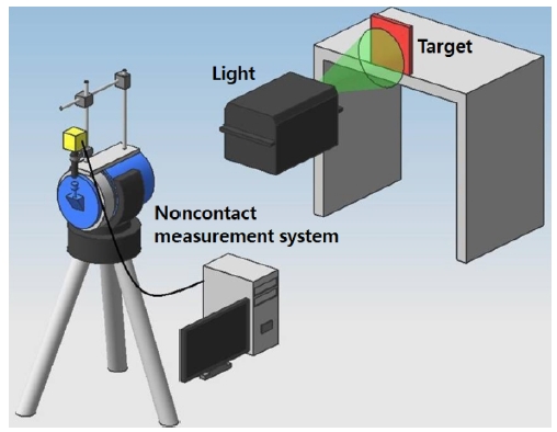
Micro-telescopic measurement system for the detection of vibratory displacements of solid bodies in long distance
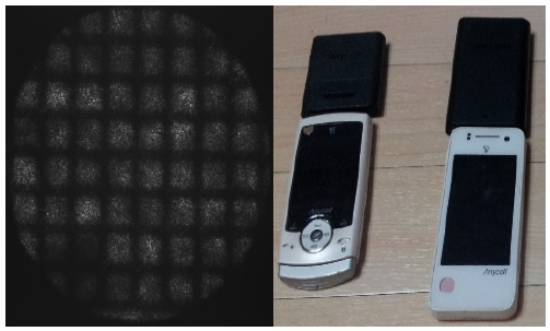
Image of the target grid and two mobile phones. The target is attached onto the mobile phone (model A, model B) for imaging.
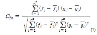
Here, fi and gi mean the image intensity of the two consecutive frames. Using this equation, the displacements of the target body were calculated. Using the coordinates of the displacement calculated from three consecutive images, the acceleration of the body can be calculated using Equation (2).

Here, (x1, y1), (x2, y2), and, (x3, y3) are the coordinate that can be calculated from the displacements.
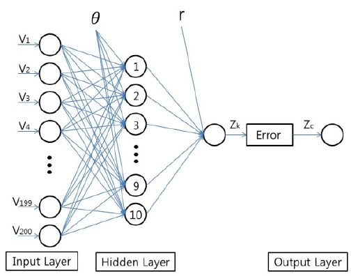
Figure 2 shows the used model of neural network. The network consists of three layers, input layer, hidden layer and output layer. The hidden layer consists of 10 neurons. The vibratory data that can be obtained from time consecutive accelerations of the target body using the PIV technique, and these data are trained for the input layer of the neural network in real time. Simultaneously, these acceleration data are also used for training the output layer. The number of data used for the input layer is changed dynamically so that real-time monitoring can be attained minimizing time loss.
3. Results and Discussions
3.1 Measurements on Transient Change of Vibration
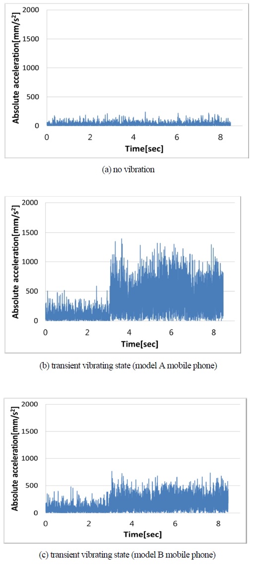
Figure 4 (a), Figure 4 (b) and Figure 4 (c) show the time history of the acceleration representing Equation (2) for three states. Figure 4 (a) shows the acceleration when there was no excitation of force. Even under no excitation, there exists acceleration. This is due to the vibration of the building where the mobile phone and the measurement system are installed. Figure 4 (b) and Figure 4 (c) show the temporal acceleration data obtained under the transient state for the model A phone and model B phone, respectively. From these two figures, it can be said that the two acceleration patterns are completely different. For the case of model A mobile phone, the abrupt change of the acceleration can be discriminate directly. However, for the case of model B, it is not so easy to say from the acceleration data that the mobile phone is under vibration state or not, because there is no conspicuous boundary between no-vibration and vibration states.
3.2 Performance Test of Real-Time Monitoring with Maximum, Mean, Minimum Values
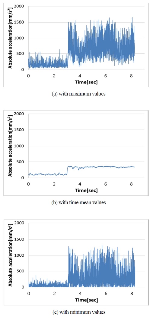
The ideal signal pattern for the identification of different vibration state of the solid body is the stepwise function shape as shown in Figure 6 (b).
Figure 5 shows the concept of real-time monitoring. The raw data of the acceleration calculated by the PIV technique were used for the training of the input layer. Simultaneously, a representative data, such as the maximum, the time-mean, and the minimum data were used for the training of the output layer. The representative data were sampled from the time consecutive acceleration data. The number of samples was adjusted for performance comparison for real-time monitoring.
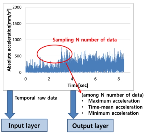
Concept of real-time monitoring. The data are used to train the neural network for real-time monitoring
Figure 6 shows the structure of sampling data that were used for training the output layer of the neural network in real time. N number of data was sampled for training at first, and the next data set was shifted to 1 data, by which all data set are the same number. Figure 7 (a), Figure 7 (b) and Figure 7 (c) show the monitoring results of the neural network in real time. Figure 7 (a) shows the monitoring results (output signals) when the maximum values of acceleration were used for training the output layer. Among 50 data, the maximum value was only used for training the output layer. In this manner, all maximum values among the next consecutive 50 sets were used for teaching the output layer. The output signals show random, from which clear prediction in real time on the working condition of the phone cannot be made. Figure 7 (b) shows the output signals when the time-mean values of acceleration were used for training the output layer. As shown in the figure, the pattern of the signal is a stepwise function and is a very clear pattern. This implies that this signal can be utilized for making a clear decision to take the next countermeasure for the solid body to be kept from an emergency circumstance or a mechanical trouble. Figure 7 (c) shows the monitoring results (output signals) when the minimum values of acceleration were used for training the output layer. It seems that the overall pattern or profiles of the each signal look like a stepwise one. However, each signal varies very randomly at each time step. This implies that this discontinuous data cannot be utilized to make a clear decision by an electric or an electronic apparatus.
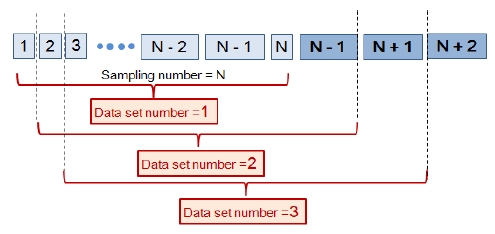
Structure of sampling data used for training the output layer. N number of the sampled data was used and 1 data was shifted to the next.
3.3 Performances Test for Different Data Number
From the above test for the three different values (maximum, time mean, minimum), it was verified that the time mean values are most appropriate one to be taught for the output layer in order to make a clear decision, by which an electronic signal can be produced so that an automatic monitoring can be achieved. By the way, there is report on the optimized number of data to be used for sampling. Jeon et. al. [6] reported that the optimal sampling number was 50. However, their case was on the case of close-view not on the case of tele-distance view. For the case of tele-measurements, the optimal sampling number should be checked. In this section, the output signals were investigated changing the number of data sampling.
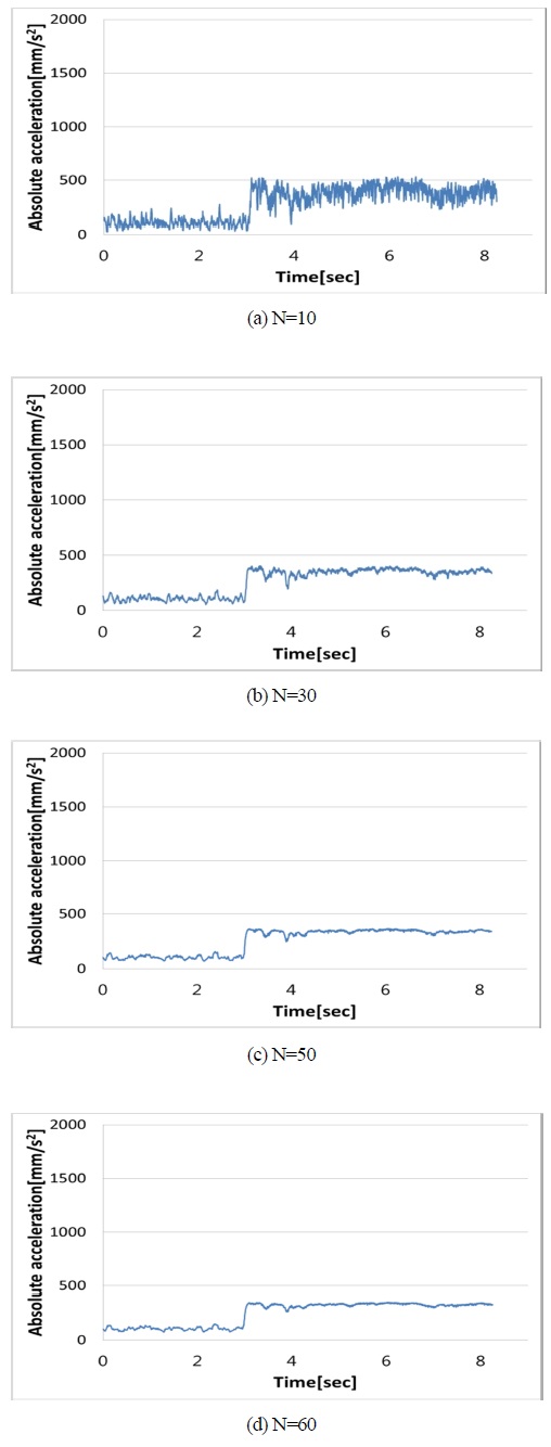
Figure 8 (a), Figure 8 (b), Figure 8 (c) and Figure 8 (d)1 show the monitoring results when the number of data sampling was set to 10, 30, 50 and 60, respectively. When the data sampling number was set to 10, the monitoring results showed very unstable signals. When the number was increased, the stepwise signals showed stable and clear pattern. This signals showed the clearest and most stable when the number was set to 60. This profile didn’t change anymore, even if the number was increased. This implies that the most appropriate data number is close to 60 for the cases of tele-measurements.
4. Conclusions
A microscopic and telescopic monitoring system for the diagnosis of the vibratory solid bodies in remote was constructed. With the system, two mobile phones were installed at tele-distances (in this study, 20meters away from the system), and the vibration of the phone was detected by the measurement system. From the experiments, the results are summarized as follows.
A neural network was adopted for real-time monitoring, in which three different types of data signals, such as maximum, mean, minimum values among the sampled data were used for real-time diagnosis on the vibratory solid body.
It was verified that time-mean value was most appropriate for realtime monitoring.
The most appropriate data sampling number was 60.
Acknowledgments
This research was supported by Basic Science Research Program through the National Research Foundation of Korea (NRF) funded by the Ministry of Education (2014R1A1A4A01005191).
This paper is extended and updated from the short version that appeared in the Proceedings of the International symposium on Marine Engineering and Technology (ISMT 2014), held at Paradise Hotel, Busan, Korea on September 17-19, 2013.
References
-
M. G. Jeon, G. R. Cho, J. S. Oh, C. J. D. Lee, and D. H. Doh, “Measurements of remote micro displacements of the piping system and a real time diagnosis on their working states using a PIV and a neural network”, Transaction of the Korean Hydrogen and New Energy Society, 24(3), p264-274, (2013).
[https://doi.org/10.7316/KHNES.2013.24.3.264]

-
K. Machida, H. Okamura, T. Hirano, and K. Usui, “Stress analysis of mixed-mode crack of homogeneous and dissimilar materials by speckle photography”, Transactions of the Japan Society of Material Engineers, 67(655), p86-91, (2001).
[https://doi.org/10.1117/12.429589]

- R. Shien, T. Numayama, S. Masumi, K. Nabara, and D. Kobayashi, “Noncontact deflection distribution measurement for large-scale structures by advanced image processing technique”, Materials Tran, 53(2), p323-329, (2012).
-
S. Braun, “The synchronous (time domain) average revisited”, Mechanical Systems and Signal Processing, 18, p1087-1102, (2011).
[https://doi.org/10.1016/j.ymssp.2010.07.016]

-
K. H. Shin, “Realization of the real-time domain averaging method using the kalman filter”, Journal of International Precision Engineering and Manufacturing, 12(3), p413-418, (2011).
[https://doi.org/10.1007/s12541-011-0053-4]

-
K. S. Son, H. S. Jeon, S. W. Han, and J. W. Park, “Enhancement of displacement resolution of vibration data measured by using camera images”, Transactions of Korean Society of Noise and Vibration Engineering, 24(9), p716-723, (2014).
[https://doi.org/10.5050/KSNVE.2014.24.9.716]

-
R. J. Adrian, “Particle-imaging techniques for experimental fluid mechanics”, Journal of Annual Review of Fluid Mechanics, 23, p261-304, (1991).
[https://doi.org/10.1146/annurev.fl.23.010191.001401]

-
D. E. Rumelhart, G. E. Hinton, and R. J. Williams, “Learning representations by back-propagating errors”, Nature, 323, p323-536, (1986).
[https://doi.org/10.1038/323533a0]

-
T. Utami, and R. A. Blackwelder, “A cross correlation technique for velocity field extraction from particulate visualization”, Experiments in Fluids, 10, p213-223, (1991).
[https://doi.org/10.1007/BF00190391]


