Adjusted k-nearest neighbor algorithm: Application on forecasting the ship accident in South Korea
Copyright © The Korean Society of Marine Engineering
This is an Open Access article distributed under the terms of the Creative Commons Attribution Non-Commercial License (http://creativecommons.org/licenses/by-nc/3.0), which permits unrestricted non-commercial use, distribution, and reproduction in any medium, provided the original work is properly cited.
Abstract
In this paper, we propose a new forecasting approach that finds a nearest-neighbor optimum for forecasting. It blends the advantages of subsample use (k-nearest neighbor, rolling window, etc.) and entire sample use. Basically, it belongs to the range of nearest neighbor methods but is different from them in that it also considers the entire sample, which can help to yield less variance in test error than other subsample methods. To improve forecasting accuracy, we also used a modified least squares method in the process of this forecasting approach. From simulation tests, we were able to verify that this approach yielded less test error than other methods that do not adopt this approach. Empirical verification using time-series data on the ship accident also supported that this approach is able to improve forecasting accuracy. In addition, we were able to verify that the test errors obtained from this approach were less than the residuals obtained from fitting using the actual future value in many cases. A new parameter controlling a weight between the subsample and the entire sample is introduced, and the forecasting performance may depend on how this parameter can be efficiently used.
Keywords:
Combination of forecast, Forecasting, Nearest neighbor searches, Pseudo data, Ship accident1. Introduction
Both entire sample and subsample use have pros and cons when used for forecasting. The former has been intensively addressed in asymptotic studies and the latter is usually seen in machine learning or related fields. From a test error point of view, the former contributes low variance to test error, the latter contributes a low bias to it, and so in most cases, unbiasedness should be assumed in the former even at the cost of high test error. Meanwhile, in the stochastic process, moving average methods adopt the nearest subsample for better forecasting, which is called rolling or sliding window. Although there are some studies on how to determine the rolling window in some specific situations [1][2], there does not seem to be a universal approach, and so the forecasting performance is sensitive to the size of the rolling window [3].
There is also a similar problem when using the k-nearest neighbor (kNN) algorithm, specifically concerning how to determine the size of k. Analogous to the problem of selecting the rolling window, it also varies depending on a given data set, and so we should experimentally estimate the optimal k value from past forecast results. There are still some technical aspects to be determined such as which form of k should be used. For example, an estimate of k may seriously vary according to the location from which it is obtained; we need to decide which to use from the average k, the most recent k, or another representative k. The degree of data dispersion (noise) is also a crucial factor for the kNN algorithm when assessing its performance on forecasting [4].
When forecasting, one may prefer nearest neighbor methods to guess a neighboring future value or use an entire sample to discover the underlying process before making the forecast. If we set a closed interval in which the initial point is kNN and the end point is the entire sample, and we can consider a linear combination of these two that can be used for the accurate forecasting. We call this adjusted k-nearest neighbor (AkNN) and searching for it is the key to more accurate forecasting and is the core idea presented in this paper.
There is another trick to improve forecasting accuracy by using pseudo data to forecast future values [5][6] based on the typical fact that training error underestimates test error [7]. If we transform test error minimization problem to training error one, we can obtain an estimate more appropriate to minimizing test error than just minimizing training error when estimating parameters. We use this technique associated with the process of finding the AkNN.
For the numerical verification of our proposed method, we used simulation data sets and real time-series data of the ship accident in South Korea. For each case, we forecast the number of the one-step ahead ship accident based on the training data. The remainder of the paper is organized as follows. The theoretical background of our forecasting method is introduced in Section 2, and Section 3 contains the verification of this approach with simulation studies and on two sets of empirical data, while conclusions and future work are covered in Section 4.
2.Methods
2.1 Nearest-Neighbor Approaches
Of the popular nearest neighbor approaches, kNN is used in the field of machine learning, and rolling window is used in the field of time series analysis.
Most studies have mainly addressed the kNN algorithm in classification or fitting, while some have adopted it for forecasting. For example, the kNN algorithm has been used to forecast future traffic flow, and the method based on the kNN algorithm gave more improved forecasting accuracy than one that was not [8]. In another study, the kNN algorithm has been combined with an SVM according to the distance from a separating hyperplane for solar flare forecasting [9]. There are also some studies using kNN on time series prediction; for example, the kNN algorithm has been applied to forecasting short-term electric energy demand and compared with a conventional dynamic regression technique [10]. An interesting approach has also been proposed to find an optimal size of nearest neighbor for time-series prediction by using multiple nearest neighbors to same data [11]. Thus, there have been many studies combining kNN algorithm with other machine learning techniques or applying it to practical areas, however it seems that there are not many studies addressing the shortcoming of it, which is caused by using only a small part of the entire sample.
In moving average methods, a rolling window refers to the size of the most recent data to forecast future values. It is similar to kNN in that it uses neighboring points, but it only considers the distance in the space of a predictor. In a moving average method, consider the time series sequence { yt }t =1,… , and when forecasting a value at t = T with rolling window n, then the moving average is
| (1) |
Based on the similarity of the nearest observations, a better forecast can be obtained than one from using a whole data set according to n, although only considering the n data may lead to a large variance. Therefore, selecting the optimal window size is a critical issue for accurate forecasting, and in many applications, it is experimentally obtained from past data. Rolling windows of different sizes were used, and the results from them were compared using an autoregressive model for forecasting the consumer price index and industry production [12], and a specific rolling window of size 68 selected out of 60-82 was used when forecasting inflation indices across five countries [13]. There have also been researchers who have tried an analytical approach on how to determine the window size. The study in [14] focused on estimating the windows size when structural breaks existed in a given stochastic process because these affected changes in the parameters to be estimated. Approaches based on geometrical characteristics to find the optimal window size have also been attempted [15]. Unlike the studies using kNN algorithm, many studies using a rolling window seem to have mainly focused on forecasting in practical areas, and so the optimal window sizes widely vary depending on the given data.
2.2 Combination for Forecasting
Test error is typically higher than training error obtained from a given data set [7]. Therefore, among forecasting-oriented studies, alleviating over-fitting plays a major role in getting an accurate forecast. Shrinkage or regularization methods in the field of machine learning such as ridge regression, lasso, etc. have been introduced to deal with the over-fitting problem. When considering the shrinkage of estimated coefficients to avoid being overly biased against one forecasting model, a combination of several forecasts can be an alternative. Consider forecasts f1, . . ., fM from M models and suppose that their variances σ1, . . ., σM are uncorrelated, then combination of forecasts fc is
| (2) |
where and . Note that the weight is inversely proportional to the forecast’s variance [16]. A combination of forecasts still yields an accurate forecast even in cases where the variances of the forecasts are correlated [17]. Furthermore, analogous to shrinkage or regularization, a unique approach was suggested to shrink fc into λc, λ < 1, giving up the sum of a combination of weights to be one for better accuracy [18]. The idea of combining forecasts is based on Jensen’s inequality [16] as long as a loss function is convex. Meanwhile, questions remain on how many forecasting methods to use and which ones work well together. We also found a different type of combination under structural change [19]. In this study, rather than combining forecasts from different models, the method here was to combine the estimated coefficients of rolling and expanding (or recursive) windows in the same forecasting model. Let and be the estimated coefficients in rolling and expanding window forecasts, respectively, then the combination coefficient is
| (3) |
where α is an optimal weight of less than 1. This approach has the advantage of not considering the choice among the forecasting models unlike the previous forecasting combination, but it is still a linear combination of already estimated parameters bounded by and , similar to the previously reported forecasting combination methods.
2.3 Least Squares Adjusted With Pseudo Data (LSPD) for Forecasting
Let us consider a data set {yt}t=1,…,T and suppose that we want to forecast yT+1. In most cases, we use estimated parameters obtained from using the T data set to forecast a future value at T+1. Unfortunately, the over-fitting problem is likely to occur in this case unless the stochastic process is a martingale, i.e., E(yT+1|yT,…, y1) = yT. If we set a pseudo value close to the future value at T+1, we can construct a loss function including the (T+1) data set rather than the T data set and obtain a better forecast using this transformation [5][6]. Hence, test error obtained from the (T+1) data set including a pseudo data point are less than test error from using the T data set,
| (4) |
where is a pseudo data point constructed from using the T data set. We can consider many candidates for this pseudo data point but in practice, the sample mean is the most appropriate based on the central limit theorem. This method provides better forecasting by just adding the pseudo data point, but its degree of improvement decreases as the data size increases.
2.4 AkNN for Forecasting
Nearest neighbor approaches can give a good approximation of a forecast but easily lead to a large variance due to using a small sample. From the forecast combination, we can obtain better forecasting accuracy by the regularization effect. Here, we propose a new forecasting method that blends subsample use and entire sample use, which is also associated with LSPD to forecast more accurately. By combining subsample use and entire sample use, we can avoid the large variance problem unlike the nearest neighbor approaches and the decrease of forecasting improvement of LSPD.
Let X and y be random variables on probability spaces ( ΩX, ΣX, μX) and ( Ωy, Σy, μy) , respectively, and consider a stochastic process (Xt, yt), for t = 1,…, T+1. Suppose that we want to forecast a future value at T+1. First, we try to find a nearest neighbor of the most recent cases to forecast this future value. Since the most recently estimated nearest neighbor varies depending on the forecasting location, its direct use or the average of the nearest neighbors over some interval may not give a stable result. To obtain a robust estimate of the nearest neighbor on a random basis, we construct bootstrap samples by b iterations and attach a pseudo value at T+1 to each sample for using LSPD. Subsequently, we obtain bootstrap samples {(Xj,t, yj,t)}, for j = 1,…, b, t = 1,…, T+1, and for T+1, a pseudo value (sample mean up to T) is used instead of the actual yT+1.
Denote the size of the nearest neighbor as kj and obtain its estimate for a forecast at t (kj < t ≤ T + 1) by minimizing test error using LSPD:
| (5) |
where Xj,‖t-kj‖ is a ‘kj ’th nearest point to Xj,t . Let kj,o be the corresponding nearest neighbor for d’ by linearly combining d and L = ‖ Xj,T+1 − Xj,1 ‖, which acquires more stability than a simple nearest neighbor. Thus,
| (6) |
where αj is a new parameter that is a nonnegative weight of less than or equal to one.
We can obtain an optimal by
| (7) |
Since is optimal for each bootstrap sample, we average over b, and then we obtain the bagged estimate
| (8) |
and by estimating (corresponding metric: do) of the original T data set, we obtain k* for the forecast at T+1 from its corresponding metric d*:
| (9) |
By using as AkNN we can expect less variance than that from a simple nearest neighbor approach and overcome a drawback of LSPD. We summarize the above procedure in the following algorithmic form.
3. Numerical results
3.1 Simulation Testing
We used three functions to examine the generalization of our method; a linear function as the basic model, a polynomial function for the sensitivity to the curve, and sine and logarithm functions as the complicated data generating process
Model 1
Model 2
Model 3
where xi is a random variable in [0,1] and is used for considering the distance in the kNN algorithm [20], and ei is an independent and identically distributed random variable orthogonal to xi and normally distributed with zero mean and unit variance.
Samples of 100 and 300 were used for each simulation test, the number of Monte Carlo iterations was 100, and the number of bootstrap subsamples was 50 (of course, the forecast accuracy increased as the number of bootstraps increased).
Table 1 shows a test error comparison for the proposed method and some previously reported methods. In general, we can see that test errors were mainly large in the order of ordinary least squares OLS, LSPD, and AkNN (the proposed method), and the results of kNN and AkNN improved when the simulation function model was more curved (non-linear). Conversely, with Model 1, their improvements were slight since the linear form was the true model. kNN did not show low test error with any of the models and obtained the highest test error in the linear case (Model 1) and the lowest in the nonlinear case (Model 3), which is as expected considering the property of kNN using only a small portion of the data. LSPD consistently outperformed OLS but its improvement became smaller as the sample size increased. We can also see that the degree of reduced test error percentage compared with OLS decreased in the LSPD case but increased in the AkNN case as the sample size increased. Note that AkNN outperformed the results of ACT (residuals from fitting when the actual value at T+1 assumed to be known) for Models 2 and 3.
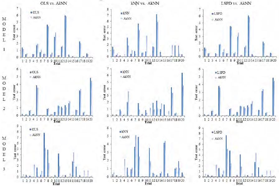
Figure 2 shows test error comparisons of AkNN with the other methods over 20 arbitrary trials. From Model 1 to Model 3, the performance of AkNN was better than its counterpart in each case although it seemed to fluctuate, which implies that kNN’s influence increased as the simulation function became more curved. A similar phenomenon is evident in the middle charts of kNN vs. AkNN, reflecting a large variance caused by kNN.
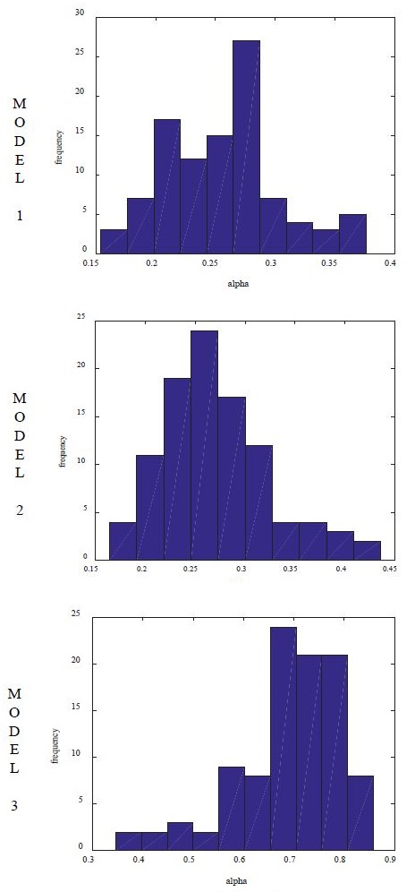
Figure 3 shows the histograms of α in Equation (8) over 100 trials. Overall, they show a bell-shaped distribution, which implies that α can be used as a parameter in each particular data generating process. From Equation (9), we can see that the greater α is, the more depends on the nearest neighbor . From Models 1-3 shown in Table 2, α becomes greater, reflecting that kNN’s influence increased.
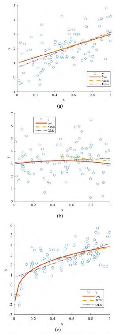
Figure 4 shows estimated lines from OLS and AkNN when both were compared with the original simulation function (y–e: noisefiltered y). We can see that AkNN uses a subsample on all the models and also that the end point, i.e. the forecast, of AkNN is closer to the end point of the original function than OLS in every case.
3.2 Empirical Study
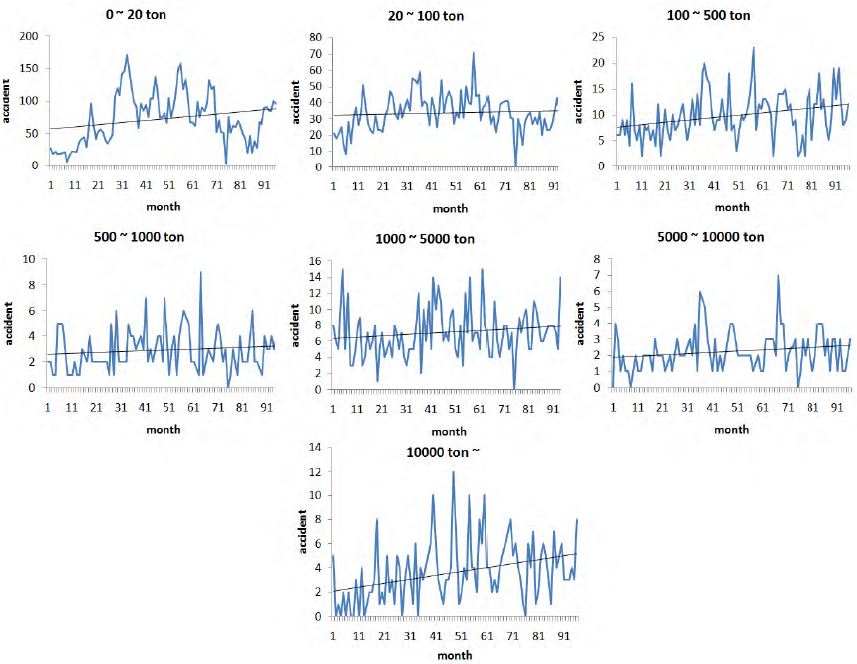
Ship accident is considered as a serious event because the emergency process is not quickly taken. Overall, the number of the ship accident is gradually increasing as shown Figure 5. There are some papers [21][22][23] studying the human factor of the ship accident, but there does not seem to be many studies on the forecasting the ship accident from a statistical point of view. Considering this point, we forecast the number of the onestep ahead ship accident based on our proposed method (AkNN), and since the number of ship accident is varied according to the ship weight, we forecasted the number of the ship accident by each weight.
We collected the 96 monthly data on the ship accident for each weight between Jan. 2000 and Dec. 2014 in South Korean waters, and the test errors from the last 40 observations were obtained and compared across the methods. The trends in Figure 5 seem to be moderate, but the degree of noise is quite high, and thus a nearest-neighbor approach will promise desirable forecasting performance.
In Table 3, the test errors of AkNN were mainly less than the rival methods, OLS, kNN, and LSPD, and in some cases, it was less than the residuals obtained from ACT in some cases. kNN showed good forecasting performances compared to OLS in some cases, but in other cases its forecasting accuracy was very low, which reflects the high variance of the subsample use and affects its high standard deviation in the table.
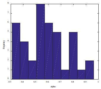
Histograms of α in the ship accident data is shown in Figure 6. Not as close to a bell shape as the simulation case, it shows a peak around the mean. The mean of alpha was 0.5820 and its standard deviation 0.1702.
4. Conclusion
We proposed a new forecasting method by combining subsample use (kNN or rolling window) and entire sample use, and parametrized a weight in a linear combination of both uses. We also added the LSPD method for better forecasting.
We were able to obtain numerical results by simulation and ship accident data to support that our forecasting method reduced test error compared with other methods and also yielded less test error than the residual obtained from the fitting using the actual future value in many cases, which also reflects the difference between test error and training error. The histogram of the weight α showed a central tendency in a bell shape, which implies that it was usable as a parameter for the given data.
The technique to find the AkNN in our proposed method can be applied to any forecasting model; for example, we could check that simple linear regression can give better forecasting results by adopting this technique. However, it still depends on the numerical method to find k-nearest neighbor, and so it needs a lot of time, which may be a restriction to apply out method to a large sample.
The new parameter α seems to be convergent, but it may be affected by the entire sample size and the degree of noise. In future work, the properties of α should be analyzed further and, its more efficient use can be presented from these analyses.
References
-
A. Inoue, L. Jin, and B. Rossi, “Rolling window selection for out-of-sample forecasting with time-varying parameters”, Journal of Econometrics, vol. 196(no. 1), p55-67, (2017).
[https://doi.org/10.1016/j.jeconom.2016.03.006]

-
T. Ouyang, X. Zha, L. Qin, Y. Xiong, and H. Huang, “Model of selecting prediction window in ramps forecasting”, Renewable Energy, vol. 108, p98-107, (2017).
[https://doi.org/10.1016/j.renene.2017.02.035]

-
B. Rossi, and A. Inoue, “Out-of-sample forecast tests robust to the choice of window size”, Journal of Business & Economic Statistics, vol. 30(no. 3), p432-453, (2012).
[https://doi.org/10.1080/07350015.2012.693850]

-
T. Yang, L. Cao, and C. Zhang, “A novel prototype reduction method for the K-nearest neighbor algorithm with K ≥ 1”, Proceedings of the 14th Pacific-Asia conference on Advances in Knowledge Discovery and Data Mining, p89-100, (2010).
[https://doi.org/10.1007/978-3-642-13672-6_10]

- J. W. Kim, and J. C. Kim, “Nonparametric forecasting with one-sided kernel adopting pseudo one step ahead data”, Proceedings of the Autumn Conference of the Korean Data and Information Science Society, p9, (2010).
-
J. W. Kim, J. C. Kim, J. T. Kim, and J.H. Kim, “Forecasting greenhouse gas emissions in the Korean shipping industry using the least squares adjusted with pseudo data”, Journal of The Korean Society of Marine Engineering, vol. 41(no. 5), p452-460, (2017).
[https://doi.org/10.5916/jkosme.2017.41.5.452]

-
T. Hastie, R. Tibshirani, and J. Friedman, The Elements of Statistical Learning, Berlin, Germany, Springer series in statistics, (2009).
[https://doi.org/10.1007/978-0-387-21606-5]

-
L. Zhang, Q. Liu, W. Yang, N. Wei, and D. Dong, “An improved K-nearest neighbor model for short-term traffic flow prediction”, Procedia - Social and Behavioral Sciences, vol. 96, p653-662, (2013).
[https://doi.org/10.1016/j.sbspro.2013.08.076]

-
R. Li, Y. Cui, H. He, and H. Wang, “Application of support vector machine combined with K-nearest neighbors in solar flare and solar proton events forecasting”, Advances in Space Research, vol. 42(no. 9), p1469-1474, (2008).
[https://doi.org/10.1016/j.asr.2007.12.015]

- A. T. Lora, J. M. R. Santos, J. C. Riquelme, A. G. Exposito, and J. L. M. Ramos, “Time-series prediction: Application to the short-term electric energy demand”, Current Topics in Artificial Intelligence Lecture Notes in Computer Science, p577-586, (2004).
- D. Yankov, D. Decoste, and E. Keogh, “Ensembles of nearest neighbor forecasts”, Lecture Notes in Computer Science Machine Learning: ECML 2006, p545-556, (2006).
-
M. Piłatowska, “Information and prediction criteria in selecting the forecasting model”, Dynamic Econometric Models, vol. 11, p21-40, (2011).
[https://doi.org/10.12775/dem.2011.002]

-
Y. C. Chen, S. J. Turnovsky, and E. W. Zivot, “Forecasting inflation using commodity price aggregates”, Journal of Econometrics, vol. 183(no. 1), p117-134, (2014).
[https://doi.org/10.1016/j.jeconom.2014.06.013]

-
M. H. Pesaran, and A. Timmermann, “Selection of estimation window in the presence of breaks”, Journal of Econometrics, vol. 137(no. 1), p134-161, (2007).
[https://doi.org/10.1016/j.jeconom.2006.03.010]

-
R. M. Kil, S. H. Park, and S. H. Kim, “Optimum window size for time series prediction”, Proceedings of 19th Annual International Conference of the IEEE engineering in medicine and biology magazine, p1421-1424, (1997).
[https://doi.org/10.1109/iembs.1997.756971]

-
J. M. Bates, and C. W. Granger, “The combination of forecasts”, Operations Research, vol. 20(no. 4), p451-468, (1969).
[https://doi.org/10.2307/3008764]

- G. Elliott, C. Granger, and A. Timmermann, Handbook of Economic Forecasting, Elsevier, North-Holland, (2006).
- T. Wenzel, The Shrinkage Approach in the Combination of Forecasts, Technical Report 44, University of Dortmund, (2000).
-
T. E. Clark, and M. W. Mccracken, “Improving forecast accuracy by combining recursive and rolling forecasts”, International Economic Review, vol. 50(no. 2), p363-395, (2009).
[https://doi.org/10.1111/j.1468-2354.2009.00533.x]

- A. Sasu, “K-nearest neighbor algorithm for univariate time series prediction”, Bulletin Of The Transilvania University Of Brasov Series. III, vol. 5(no. 54), p147-152, (2012).
-
D. J. Kim, and S. Y. Kwak, “Evaluation of human factors in ship accidents in the domestic sea”, Journal of the Ergonomics Society of Korea, vol. 30(no. 1), p87-98, (2011).
[https://doi.org/10.5143/jesk.2011.30.1.87]

-
H. T. Kim, S. Na, and W. H. Ha, “A case study of marine accident investigation and analysis with focus on human error”, Journal of the Ergonomics Society of Korea, vol. 30(no. 1), p137-150, (2011).
[https://doi.org/10.5143/jesk.2011.30.1.137]

-
C. Chauvin, S. Lardjane, G. Morel, J.P. Clostermann, and B. Langard, "Human and organisational factors in maritime accidents: Analysis of collisions at sea using the HFACS", Accident Analysis & Prevention, vol.59, p26-37, (2013).
[https://doi.org/10.1016/j.aap.2013.05.006]


