Mapping predicted carbon dioxide emissions from ships using gradient-boosting-based models
Copyright © The Korean Society of Marine Engineering
This is an Open Access article distributed under the terms of the Creative Commons Attribution Non-Commercial License (http://creativecommons.org/licenses/by-nc/3.0), which permits unrestricted non-commercial use, distribution, and reproduction in any medium, provided the original work is properly cited.
Abstract
Monitoring the amount of CO2 emitted by individual ships in real-time is currently impossible. Therefore, we conducted a study to predict and map CO2 emissions using gradient boosting-based models trained based on ship data and emission data collected from ships. The extreme gradient boosting (XGBoost) and light gradient-boosting machine (LightGBM) models were used, and a hyperparameter tuning process was performed to improve the model performance. The results confirmed that hyperparameter optimization improves model performance. Based on these models, CO2 emissions were predicted and expressed in a map with black, red, orange, and yellow colors, according to the range of CO2 emissions for the three voyages, consequently confirming that the ship itself or the ship management company can monitor CO2 emissions from ships by mapping them on a global map.
Keywords:
Mapping, Carbon dioxide, Gradient boosting, XGBoost, LightGBM1. Introduction
Ship emissions affect the environment, economy, and human health. Environmental damage includes climate change caused by greenhouse gases (GHG) such as carbon dioxide (CO2), methane (CH4), and nitrous oxide (N2O) [1][2]. Climate change affects the weather (higher average temperatures, longer-lasting droughts, more intense wildfires, and stronger storms), environ-ment (melting sea ice, sea level rise, flooding, warmer ocean waters and marine heat waves, and ecosystem stressors), agricul-ture (less predictable growing seasons, reduced soil health, and food shortages), animals, and humans (human health, worsening inequity, displacement, and economic impacts) [3]. As CO2 ac-counts for the largest proportion of greenhouse gas (GHG) emis-sions, research and policies to reduce it are actively underway. Internationally, efforts have focused on regulating GHG emis-sions from ships by introducing the existing energy efficiency ship index (EEXI) and carbon intensity indicator (CII) [4]. Fur-thermore, research is actively being conducted on eco-friendly fuels such as ammonia, methanol, and hydrogen, and post-treatment processes such as CO2 capture system (carbon capture, utilization, and storage (CCUS)) [5]-[7].
Economic damage includes carbon taxes caused by ship emissions and damage caused by natural disasters due to global warming. Human health damage includes premature deaths ow-ing to global shipping-sourced emissions [8]. Therefore, moni-toring ship emissions and implementing appropriate measures to reduce them is crucial. However, installing equipment to measure ship emissions is not common owing to high equipment costs and less stringent regulations.
To address this issue, studies have focused on predicting emis-sions using machine learning (ML)-based methods. Yang et al. predicted GHG emissions with 92.5% accuracy based on the sailing speed, displacement, and weather conditions in an oil tanker noon report [9]. Lee et al. predicted fuel consumption and carbon emissions using random forest, LightGBM, and long short-term memory (LSTM) based on the operation data of dual-fuel propulsion ships [10]. Cao et al. predicted fuel sulfur content using an ultraviolet image of an exhaust plume obtained from an ultraviolet camera and a convolutional neural network [11]. Reis et al. used regression models based on profile-driven features and statistical pattern analysis to predict the CO2 emissions of Ro-Pax ships sailing medium and long routes [12]. Liu and Duru developed a Bayesian ship traffic generator to overcome the limi-tation of the inability to identify future ship movements, with ship emission forecasts generated accordingly [13]. Lepore et al. compared and analyzed several regression techniques to predict CO2 emissions [14]. In addition to focusing on emissions predic-tion, research on emissions mapping is actively underway.
Buber et al. used point density analysis in MapInfo v.16 to represent the spatial distribution of emissions from domestic shipping [15]. Topić estimated the CO2 emissions of container-ship traffic for a year using statistical energy analysis methodolo-gy and expressed this on a spatial map [16]. Huang et al. ex-pressed the annual NOx emissions from ships as spatial distribu-tions using traditional and dynamic methods [17]. However, no study has predicted or mapped the emissions generated from ships in real time. Therefore, in this study, we created a model to predict emissions using ML technologies based on big data col-lected from ships and then mapped these emissions accordingly. Section 2 describes ship specifications, sailing routes, and data acquisition. Section 3 describes the gradient-boosting-based algo-rithms—extreme gradient boosting (XGBoost) and light gradi-ent-boosting machine (LightGBM). Section 4 describes data preprocessing, model training, and hyperparameter optimization. Section 5 discusses the results of hyperparameter optimization, prediction results, and mapping of the predicted emissions. Sec-tion 6 summarizes the results.
2. Data Acquisition
2.1 Ship Specifications and Sailing Routes
The test object used to predict the emissions in this study was a recently built training ship. The training ship, built in 2019, is equipped with a data acquisition (DAQ) system that automatical-ly collects information from the sensors of various marine ma-chinery. The main specifications of the training ship are listed in Table 1.
The training ship, shaped like a cruise ship, is equipped with an electronic control main engine (M/E) from MAN E-S, with the long shaft installed according to the training ship structure.
The training ship sails periodically to train future navigators and engineers, with the routes on which the data are used in this study described in Table 2.
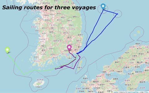
The training ships sailed to Masan, Incheon, and Ulleungdo at monthly intervals from April to June 2022. The sailing route for each voyage is illustrated in Figure 1. Global positioning system (GPS) information was collected for each voyage, and the sailing routes were displayed according to latitude and longitude, as shown in Figure 1.
In Figure 1, blue, purple, and green represent the Ulleungdo, Masan, and Incheon voyages, respectively. All voyages began in Busan, where the training ship was located.
2.2 Data Acquisition
The data collected in the DAQ system for each voyage were converted to a CSV file format. CO2 emission data were collected using a Testo 350 instrument, and the final dataset was created by merging data from the same time as the CSV file collected from DAQ.
The data for the Masan, Incheon, and Ulleungdo voyages con-sist of 292 rows and 211 columns, 305 rows and 211 columns, The data for the Masan, Incheon, and Ulleungdo voyages con-sist of 292 rows and 211 columns, 305 rows and 211 columns, and 943 rows and 211 columns, respectively. The rows represent data by time, and the columns represent the variables for the sen-sors.
However, as not all 211 variables were related to CO2 emis-sions, variables unrelated to CO2 emissions based on marine engineering field experience were excluded. With information available on the exhaust gas outlet temperature of all six cylinders in the variables, their averages were calculated and designated as a new variable to avoid data redundancy.
As a result, the following variables were selected as final input variables: (1) M/E scavenge air receiver inlet pressure, (2) M/E scavenge air receiver temperature, (3) M/E turbocharger (T/C) exhaust gas inlet temperature, (4) M/E T/C exhaust gas outlet temperature, (5) M/E revolutions per minute (rpm), (6) M/E T/C rpm, (7) M/E fuel (governor) index, (8) M/E load, (9) Shaft power, (10) M/E fuel consumption, (11) Speed log, (12) Average mean indicated pressure, (13) Average maximum cylinder pres-sure, (14) Average cylinder compression pressure, (15) M/E cylinder exhaust gas outlet temperature.
The largest portion of the emissions from ships is generated from the M/E because the M/E consumes the most fuel oil to propel the ship and produces the largest amount of energy.
The M/E was started with compressed air, and high-pressure air sequentially entered the cylinder according to the firing order of the air distributor, thereby initiating the reciprocating move-ment of the M/E. In an M/E starting with pressurized air, a com-bustion occurs within the cylinder owing to fuel injection, and the M/E gains rotational power through continuous combustion. The exhaust gas generated by the combustion of the air and fuel mix-ture passes through the T/C before being discharged into the atmosphere through a funnel. The T/C compressor pressurizes the air and sends it to an air cooler. Pressurized and cooled air passes through the air receiver and enters the cylinder of the M/E. These input variables are selected based on the M/E operation process. Among the input variables, (7)–(11) were correlated with CO2 emissions, numbers (12)–(14) were variables repre-senting the M/E performance, and (15) was the average value of the exhaust gas temperatures of the six cylinders.
3. Gradient Boosting-Based Algorithms
Gradient boosting is a technique applied to decision tree-based algorithms. This method creates a strong ensemble model by considering the decision tree as a weak learner and continuously training it using gradient descent to minimize the error between the actual and predicted values. In other words, each new deci-sion tree is trained based on the errors of the previous decision tree. Representative algorithms based on gradient boosting in-clude DMLC XGBoost and Microsoft's LightGBM [18][19].
3.1 XGBoost
XGBoost uses classification and regression trees (CART) as its base classifier, solves both regression and classification prob-lems, and uses user-created objective functions [20].
Original gradient boosting builds decision trees in series, whereas XGBoost builds them parallelly [21]. Simultaneously, the newly created decision trees predict the residuals of the previ-ous decision trees and use them for the final prediction. The gra-dient descent algorithm minimizes loss when adding newly creat-ed decision trees [22]. XGBoost surpasses existing gradient-boosting models in terms of high computing speed, expandabil-ity, and performance [23].
3.2 LightGBM
LightGBM uses gradient-based one-sided sampling (GOSS) and mutually exclusive feature bundling (EFB). The traditional method uses the level-wise method to reduce training data, whereas LightGBM uses the leaf-wise method [24]. GOSS splits the optimal nodes by calculating the variance gain, whereas EFB increases the training speed by bundling many exclusive features into fewer dense features [25]. LightGBM has the advantages of fast training speed, high accuracy, GPU learning, handling large datasets, and reducing memory occupation [26].
4. Modeling
4.1 Data Preprocessing
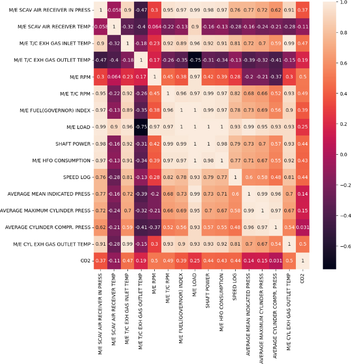
The Masan, Incheon, and Ulleungdo datasets were combined to create the total dataset, with a heat map created (Figure 2) to confirm the correlation between the input and output variables for the total dataset. Considering the output variable CO2 is on the right side of the correlation heatmap, its correlation with the input variables can be verified. Referring to Figure 2, the “M/E scav-enge air receiver temperature” and “average cylinder compression pressure” were removed because they had low correlations with CO2.
The total dataset was divided into training, validation, and test-ing sets at a ratio of 6/2/2, with the data randomly shuffled during the division.
4.2 Model training
The XGBoost and LightGBM models were trained on the training set using default hyperparameters. Performance metrics of mean absolute error (MAE), R2, and mean absolute percentage error (MAPE) were used to evaluate the performance of the trained models; their equations are listed in Table 3 [27].
The prediction results for the training, validation, and testing sets of the trained models are listed in Table 4. Both models had high-performance metrics in the order of training, validation, and testing sets. When comparing the performances of XGBoost and LightGBM, XGBoost exhibited a higher performance for all datasets.
4.3 Hyperparameter Optimization
XGBoost and LightGBM have various hyperparameters, and their model performance improves depending on their optimal combination. Therefore, this study uses the weight and bias (W&B) library, which performs the hyperparameter optimization process.
Considering XGBoost and LightGBM are gradient-boosting-based algorithms that share similar hyperparameters, hyperpa-rameters common to both algorithms were selected for optimiza-tion. The selected hyperparameters and their ranges are listed in Table 5.
“Learning_rate” sets how much previous results are reflected at each learning stage. “N_estimators” or “Num_iterations” is the number of decision trees. “Subsample” is the data sampling rate for each decision tree. “Colsample_bytree” is the feature sam-pling rate for each decision tree. “Max_depth” is the maximum depth of the decision tree. “Min_child_weight” is the minimum sum of weights for all observations required in child.
In the W&B optimization process, the range of hyperparame-ters was set, and optimization was performed 100 times by ran-dom search, aiming to minimize the MAE.
5. Result and Discussion
5.1 Results of Hyperparameter Optimization
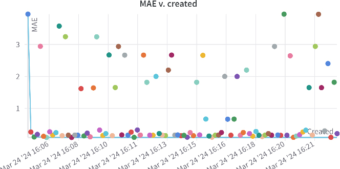
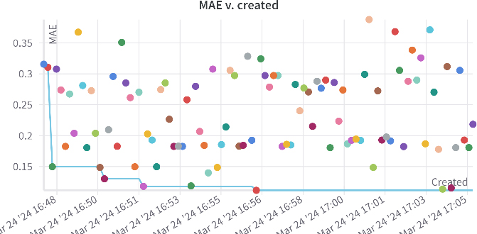
Figures 3 and 4 show the MAE performances of XGBoost and LightGBM over time, respectively. The MAE values are inconsistent because the hyperparameters are tuned using a ran-dom search method in the W&B library. Comparing XGBoost and LightGBM, XGBoost performed better for more hyperpa-rameter combinations than LightGBM, suggesting that the XGBoost model exhibits higher overall performance than the LightGBM model for the data and hyperparameter range used in this study.
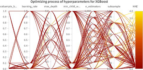
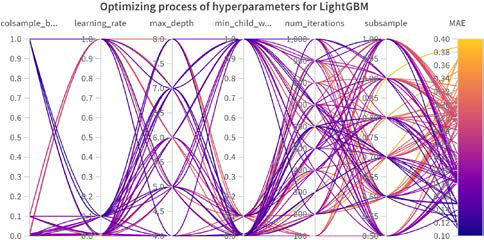
Figures 5 and 6 show the hyperparameter tuning processes of the two models in parallel coordinate plots. As confirmed in Figures 3 and 4, most of the hyperparameter combinations in Figure 5 show that the MAE converges to nearly zero, and in Figure 6, they appear to have various MAE ranges. Considering the parallel coordinate plot displays the results of hyperparameter tuning in real-time as a colored line, initially setting the hyperpa-rameter ranges would help developers.
Table 6 shows hyperparameter combinations with the lowest MAE for the validation set as a result of hyperparameter tuning. The two models shared the same hyperparameters for “Learn-ing_rate” and “Colsample_bytree,” and similar hyperparameters for “Subsample” and “Max_depth.” However, “N_estinators” and “Min_child_weight” showed conflicting results.
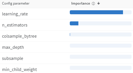
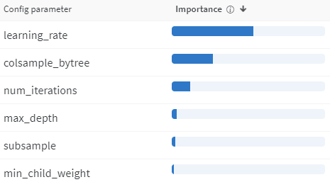
Figures 7 and 8 show the importance of the parameters in the two models. Parameter importance represents the feature im-portance values for the model by training the model with hyperparameters as inputs and the performance metric as the target output.
The parameter importance results showed that for both mod-els, “Learning_rate” was the most important for MAE. Further-more, “N_estimators” or “Num_iterations” were also shown to be important for MAE. The “Colsample_bytree” was more im-portant than “Num_iterations” in LightGBM and followed “N_estimators” in XGBoost. Considering our model was trained based on big data, “N_estimators,” i.e., the number of trees, was important in hyperparameter optimization. In terms of the overall parameter importance of the two models, the order of importance was similar.
5.2 Prediction Results of Optimized XGBoost and LightGBM
Table 7 compares the performances of the training, validation, and testing sets using the two models to which the optimal hy-perparameters obtained in Table 6 were applied. Both models exhibited high performance on the training, validation, and testing sets for all performance metrics.
Compared to Table 4, which shows the results of models trained with default hyperparameters, Table 7, with optimized hyperparameters, showed a higher performance for all perfor-mance metrics and datasets, confirmed by referring to the per-centage values of the difference in the performance metrics be-tween Tables 4 and 7. This result shows that hyperparameter optimization is essential for improving model performance.
5.3 Mapping of Predicted Emissions by Optimized XGBoost and LightGBM
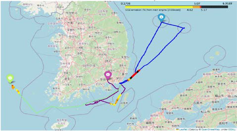
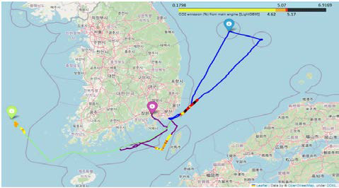
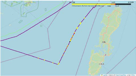
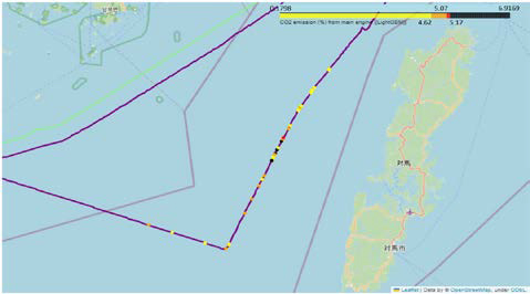
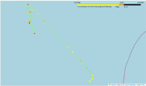
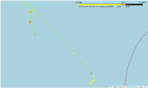
A range of CO2 emissions values was used to map predicted CO2 emissions. The CO2 range refers to the minimum (0.1798%) and maximum (6.9169%) CO2 values and quartiles of 25% (4.62%), 50% (5.07%), and 75% (5.17%) of the CO2 values in the total dataset.
Figures 9 and 10 show the mapping of CO2 emissions pre-dicted by XGBoost and LightGBM for the three voyages. The color bar at the top right indicates the range of CO2 emissions and the highest CO2 emissions in the order of black, red, orange, and yellow.
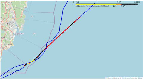
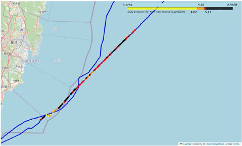
The Folium library has a scroll function to provide an overall view, as shown in Figures 9 and 10, with the enlarged maps shown in Figures 11 and 12. Figures 11 and 12, which show the CO2 emissions for the Ulleungdo voyage, indicate that the two models show similar overall predictions. With overall CO2 emis-sions mostly in red and black, considerable CO2 emissions oc-curred on this voyage.
Figure 13 and 14 present the CO2 emission mapping for the Masan voyage; while both models show CO2 emissions with orange and yellow colors, they also show black and red colors of CO2 emissions at some middle points.
Figures 15 and 16 present the CO2 emission mapping for the Incheon voyage, indicating most of the CO2 emissions were orange- and yellow-colored. With this route, emissions were considered reduced because of the complete combustion of the fuel injected into the M/E.
5.4 Limitations and Suggestions for Future Work
The proposed model was based on big data and applied to a single ship. Therefore, a certain amount of time is required to collect big data from a ship, and an update process to train the model with the additional collected data is necessary. Future work should focus on developing a model that can be used universally for multiple ships and on methods to update the model using continuously collected data.
6. Conclusion
Considering that CO2 emissions from ships can cause various environmental, economic, and human health problems, monitor-ing CO2 emissions on the ship itself or by a ship management company will become important in the future when eco-friendliness is emphasized. Therefore, we conducted a study to predict CO2 emissions and mapped them using gradient boost-ing-based models.
Vessel and emission data collected for the Masan, Ulleungdo, and Incheon voyages, each a month apart from April to June 2022, were converted into a total dataset through preprocessing, with the total dataset divided into training, validation, and testing sets in a ratio of 6/2/2.
The XGBoost and LightGBM models were trained using the default hyperparameters, with their performance evaluated using the hyperparameters optimized using the W&B library. As a re-sult, MAE/R2/MAPE for the XGBoost and LightGBM testing sets were 0.1394/0.8388/0.0782 and 0.1782/0.8068/0.0698, respectively, indicating that the performance of the optimized model was superior to that of the models with the default hy-perparameters.
CO2 emissions were predicted by the optimized models, cate-gorized by quartile range, and expressed in black, red, orange, and yellow, in the order of the highest CO2 emissions. The mapped CO2 emissions could be checked using an overall view and an enlarged view, thus allowing the ship itself or the ship management company to monitor its CO2 emissions.
Acknowledgments
This research was supported by the Autonomous Ship Technology Development Program [20016140] funded by the Ministry of Trade, Industry, & Energy (MOTIE, Korea); and the National Research Foundation of Korea (NRF) grant funded by the Korea government (MSIT) [NRF-2022R1F1A1073764]; and the Korea Maritime & Ocean University Research Fund in 2023.
Author Contributions
Conceptualization, Formal analysis, Investigation, Methodology, Data curation, Software, Visualization, Writing – original draft, Writing - review & editing, M. H. Park; Methodology, Data curation, Q. D. Vuong; Conceptualization, Data curation, Supervision, J. J. Hur; Conceptualization, Data curation, B. D. Yea; Conceptualization, Supervision, Project administration, Funding acquisition, Writing - review & editing, W. J. Lee.
References
-
D. -J. Hwang, “A study on the estimation of greenhouse gas emissions from ships according to the Tier 1 and Tier 3 methodology,” Journal of the Korean Society of Marine En-gineering, vol. 43, no. 4, pp. 292-298, 2019 (in Korean).
[https://doi.org/10.5916/jkosme.2019.43.4.292]

-
S. H. Jung, J. -H. Kim, S. -W. Kim, and J. Cheon, “Study on characteristics of GHG life cycle assessment for alterna-tive marine fuels,” Journal of Advanced Marine Engineering and Technology, vol. 45, no. 6, pp. 334-338, 2021.
[https://doi.org/10.5916/jamet.2021.45.6.334]

- Courtney Lindwall, What Are the Effects of Climate Change?, https://www.nrdc.org/stories/what-are-effects-climate-change#weather, , Accessed October 24, 2022.
-
M. Akturk and J. K. Seo, “The feasibility of ammonia as marine fuel and its application on a medium-size LPG/ammonia carrier,” Journal of Advanced Marine Engi-neering and Technology, vol. 47, no. 3, pp. 143-153, 2023.
[https://doi.org/10.5916/jamet.2023.47.3.143]

-
Q. H. Nguyen, P. A. Duong, B. R. Ryu, and H. Kang, “A study on performances of SOFC integrated system for hy-drogen-fueled vessel,” Journal of Advanced Marine Engi-neering and Technology, vol. 47, no. 3, pp. 120-130, 2023.
[https://doi.org/10.5916/jamet.2023.47.3.120]

-
K. W. Chun, “Technical guide for materials of containment system for hydrogen fuels for ships,” Journal of Advanced Marine Engineering and Technology, vol. 46, no. 5, pp. 212-217, 2022.
[https://doi.org/10.5916/jamet.2022.46.5.212]

-
H. M. Baek, W. J. Kim, M. K. Kim, and J. W. Lee, “Prepa-ration for the greenhouse gas emission issues in the national defense,” Journal of Advanced Marine Engineering and Technology, vol. 46, no. 5, pp. 277-289, 2022.
[https://doi.org/10.5916/jamet.2022.46.5.277]

-
C. Chen, E. Saikawa, B. Comer, X. Mao, and D. Ruther-ford, “Ship emission impacts on air quality and human health in the Pearl River Delta (PRD) region, China, in 2015, with projections to 2030,” GeoHealth, vol. 3, no. 9, pp. 284-306, 2019.
[https://doi.org/10.1029/2019GH000183]

-
L. Yang, L. Wei, and L. Zhang, “Thermal compensation design of truss structure for large-scale off-axis three-mirror space telescope,” Optical Engineeing, vol. 58, no. 2, 2019.
[https://doi.org/10.1117/1.OE.58.2.023109]

-
J. Lee, J. Eom, J. Park, J. Jo, and S. Kim, “The development of a machine learning-based carbon emission prediction method for a multi-fuel-propelled smart ship by using onboard measurement data,” Sustainability, vol. 16, no. 6, p. 2381, 2024.
[https://doi.org/10.3390/su16062381]

-
K. Cao, Z. Zhang, Y. Li, W. Zheng, and M. Xie, “Ship fuel sulfur content prediction based on convolutional neural net-work and ultraviolet camera images,” Environmental Pollu-tion, vol. 273, 2021.
[https://doi.org/10.1016/j.envpol.2021.116501]

-
M. S. Reis, R. Rendall, B. Palumbo, A. Lepore, and C. Capezza, “Predicting ships’ CO2 emissions using feature-oriented methods,” Applied Stochastic Models in Business and Industry, vol. 36, no. 1, 2020.
[https://doi.org/10.1002/asmb.2477]

-
J. Liu and O. Duru, “Bayesian probabilistic forecasting for ship emissions,” Atmospheric Environment, vol. 231, 2020.
[https://doi.org/10.1016/j.atmosenv.2020.117540]

-
A. Lepore, M. S. dos Reis, B. Palumbo, R. Rendall, and C. Capezza, “A comparison of advanced regression techniques for predicting ship CO2 emissions,” Quality Reliability En-gineering International, vol. 33, no. 6, 2017.
[https://doi.org/10.1002/qre.2171]

-
M. Buber, A. C. Toz, C. Sakar, and B. Koseoglu, “Mapping the spatial distribution of emissions from domestic shipping in Izmir Bay,” Ocean Engineering, vol. 210, 2020.
[https://doi.org/10.1016/j.oceaneng.2020.107576]

- Topić T, A Ship Emission Estimation Methodology with Spatial Mapping Capability for Assessing Regulation Effec-tiveness, 2022.
-
Z. Huang, Z. Zhong Z, Q. Sha, et al., “An updated model-ready emission inventory for Guangdong Province by in-corporating big data and mapping onto multiple chemical mechanisms,” Science of the Total Environment, vol. 769, 2021.
[https://doi.org/10.1016/j.scitotenv.2020.144535]

- DMLC, XGBoost.
- Microsoft Corporation, LightGBM. 2023.
-
M. Ma, G. Zhao, B. He, et al., “XGBoost-based method for flash flood risk assessment,” Journal of Hydrology, vol. 598, 2021.
[https://doi.org/10.1016/j.jhydrol.2021.126382]

-
J. Nobre and R. F. Neves, “Combining principal component analysis, discrete wavelet transform and XGBoost to trade in the financial markets,” Expert Systems with Applications, vol. 125, 2019.
[https://doi.org/10.1016/j.eswa.2019.01.083]

-
M. H. Park, S. Chakraborty, Q. D. Vuong, et al., “Anomaly detection based on time series data of hydraulic accumulator,” Sensors, vol. 22, no. 23, 2022.
[https://doi.org/10.3390/s22239428]

-
M. H. Park, J. J. Hur, W. J. Lee, “Prediction of oil-fired boiler emissions with ensemble methods considering varia-ble combustion air conditions,” Journal of Cleaner Produc-tion, vol. 375, 2022.
[https://doi.org/10.1016/j.jclepro.2022.134094]

-
Y. Ju, G. Sun, Q. Chen, M. Zhang, H. Zhu, M. U. Rehman, “A model combining convolutional neural network and lightGBM algorithm for ultra-short-term wind power fore-casting,” IEEE Access. Vol. 7, 2019.
[https://doi.org/10.1109/ACCESS.2019.2901920]

-
C. Chen, Q. Zhang, Q. Ma, and B. Yu, “LightGBM-PPI: Predicting protein-protein interactions through LightGBM with multi-information fusion,” Chemometrics and Intelli-gent Laboratory Systems, vol. 191, 2019.
[https://doi.org/10.1016/j.chemolab.2019.06.003]

-
M. H. Park, J. J. Hur, and W. J. Lee, “Prediction of diesel generator performance and emissions using minimal sensor data and analysis of advanced machine learning techniques,” Journal of Ocean Engineering and Science, 2023.
[https://doi.org/10.1016/j.joes.2023.10.004]

-
M. H. Park, C. M. Lee, A. J. Nyongesa, et al., “Prediction of emission characteristics of generator engine with selective catalytic reduction using artificial intelligence,” Journal of Marine Science and Engineering, vol. 10, no. 8, 2022.
[https://doi.org/10.3390/jmse10081118]


