Hybrid control of a tricycle wheeled AGV for path following using advanced fuzzy-PID
1Department of Mechanical r& Automotive Engineering, Pukyong National University 2Department of Mechanical r& Automotive Engineering, Pukyong National University 3Department of Mechanical r& Automotive Engineering, Pukyong National University 4Department of Mechanical r& Automotive Engineering, Pukyong National University
Copyright © The Korean Society of Marine Engineering
This is an Open Access article distributed under the terms of the Creative Commons Attribution Non-Commercial License (http://creativecommons.org/licenses/by-nc/3.0), which permits unrestricted non-commercial use, distribution, and reproduction in any medium, provided the original work is properly cited.
This paper is about control of Automated Guided Vehicle for path following using fuzzy logic controller. The Automated Guided Vehicle is a tricycle wheeled mobile robot with three wheels, two fixed passive wheels and one steering driving wheel. First, kinematic and dynamic modeling for Automated Guided Vehicle is presented. Second, a controller that integrates two control loops, kinematic control loop and dynamic control loop, is designed for Automated Guided Vehicle to follow an unknown path. The kinematic control loop based on Fuzzy logic framework and the dynamic control loop based on two PID controllers are proposed. Simulation and experimental results are presented to show the effectiveness of the proposed controllers.
Keywords:
Automated guide vehicle, Fuzzy logic controller, Path following, Dynamic modeling, Wheel mobile robot1. Introduction
Automated Guided Vehicle (AGV) is a transportation vehicle automatically traveling on unknown path traced in working environment. AGV is most often used to deliver materials around a manufacturing facility or a warehouse. With lots advantages such as reduction in the number of worker, improvement of productivity and quality, improvement of working environment and safety, less damage on transporting goods, real- time control of material flow and improved management on product, AGV has become more and more popular and useful in modern industrial production.
Control of AGV for path following has received a great of interest to many researchers because of its nonlinear characteristics caused by nonholonomic constraints of the wheels. Most controllers are designed based on nonlinear techniques [1]-[4] including the backstepping approach, the sliding mode control, the Lyapunov function approach, the dynamic feedback linearization technique, etc.. Designing controllers using these approaches is rather complex. Furthermore, it requires some detailed information related to system parameters, working environment and complete knowledge of the dynamics that are usually infeasible in practical.
To overcome the above problems, Fuzzy controller is a suitable solution. Fuzzy controller doesn’t require accuracy mathematical modeling of the system. Fuzzy logic controller can control the system with various situations of practical fields. Applying a fuzzy controller is simple, rapid and inexpensive because the rules can be linguistically interpreted by a human expert. Over the latest decade, fuzzy logic has been widely used for mobile robot control [5]-[17]. Precup et al. introduced fuzzy control solution for a class of tricycle mobile robots [11]. The control system structure contained two control loops to control the forward velocity and the direction of the robot. Antonelli et al. proposed a path following approach for mobile robot using fuzzy-logic set of rules which imitated the human driving behavior [12]. Baturone et al. introduced a design of embedded DSP-based fuzzy controllers for autonomous mobile robots [16]. In previous papers addressing path tracking control, the fuzzy controller used very simple rules and was usually single input single output controller [11], while a tricycle WMR needs a multi-input multi-output controller because it has two degree of freedom.
Among 5 types of WMR introduced by Campion et al. [18], a tricycle WMR is most widely used for industrial AGV [19]-[20]. However, a detailed report about kinematic and dynamic modeling of tricycle WMR has not been reported in literature.
From the above reasons, the purpose of this paper is as follows: First, kinematic and dynamic modeling using the well known Lagrange equation of the AGV is presented. Second, a hybrid controller that integrates two control loops, kinematic control loop and dynamic control loop, is designed for AGV to follow an unknown path. The kinematic control loop is based on fuzzy logic framework and the dynamic control loop is based on two PID controllers. For path following, a tracking error vector is defined. The fuzzy controller uses the tracking error vector as its inputs including position error, angle error and derivative of angle error. From the fuzzy output, velocity control vector at the tracking point is achieved. Because the AGV is driven by a steering driving wheel, steering angle and angular velocity of steering wheel should be calculated. Finally, in dynamic control loop, two PID controllers are used to control two DC motors for tracking the desired steering angle and the desired angular velocity of the steering wheel. Simulation and experimental results are presented to show the effectiveness of the proposed controllers.
2. System Modeling
This chapter presents the kinematic and dynamic modeling for the proposed AGV system. This AGV model is based on the model for tricycle wheeled mobile robot introduced by Campion et al. [18].
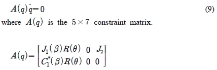
The AGV has two fixed passive wheels and one steering driving wheel. rf is the radius of two fixed passive wheel and rs is the radius of the steering driving wheel. Figure 1 shows the coordinate of AGV. XOY is the global coordinate frame and XQQYQ is the moving coordinate frame. Q is the tracking point that is placed in the middle of two fixed passive wheels. θ is the heading angle of AGV. B1 denotes a steering driving wheel.

Coordinate for AGV’s modeling
B2 and B3 denote two fixed passive wheels. XQ axis of moving coordinate frame is passed through the centers of wheels. C is the center of mass of the AGV. ϕi (i = 1,2,3) is the rotational angle of the ith wheel. β is the steering angle of the steering wheel.
The posture vector of the tracking point Q on the AGV is specified as follows:

where (x, y) are global coordinate of tracking point and θ is the heading angle of the AGV. Velocity control vector at the tracking point Q is defined as follows:

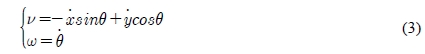
where ν and ω are linear velocity and angular velocity at the tracking point Q.
The posture vector for total AGV is specified as follows:

where Φ = [ϕ1ϕ2ϕ3]Τ. Because the AGV is driven by steering driving wheel, kinematic control vector uk is defined as follows:
2.1 Kinematic modeling
The contact between the wheels and the ground is supposed to satisfy the pure rolling without slipping condition. This means that the velocity of the contact point is equal to zero and implies that the components of this velocity parallel and orthogonal to the plane of the wheel are equal to zero. With this description, two following constraints are reduced from three wheels of AGV. Along the wheel plane (pure rolling condition):
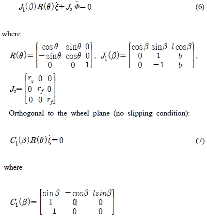
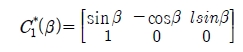
It is easy to check that rank(C1(β)) - 2. Therefore, the two last components of Equation (7) are equivalent. Without loss of generality, by removing one of two equivalent constraints, C1(β)becomes:
The corresponding constraint for no slipping condition Equation (7) is rewritten into:

From Equation (6) and Equation (8), the following constraint equation is obtained.
The constraint Equation (8) implies that the vector
 belongs to the null space of the matrix
 as follows:

This is equivalent to the following statement. For all time, there exists a time varying scalar η(t) such that the following equation is satisfied:
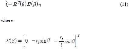
From Equation (6) and Equation (11), the following equation is obtained.
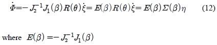
From Equation (5), Equation (11) and Equation (12), the configuration kinematic model is given as follows:
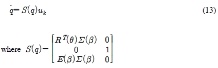
From Equation (3) and Equation (11), the velocity control vector at the tracking point Q, u is given by:
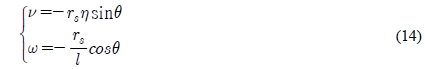
From Equation (14), the kinematic control vector uk can be achieved form u as follows:
2.2 Dynamic Modeling
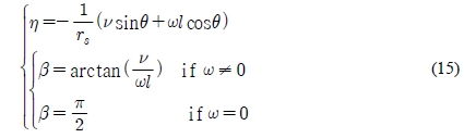
The potential energy is zero since it is assumed that the AGV is moving on a horizontal plane. The friction energy is ignored. Thus, the total kinetic energy of the AGV is given by [18].
M* : mass of the AGV without mass of wheels,
mi : mass of wheel i,
h : distance between the reference poiQnt and the center of mass C,
I0 : moment of the AGV without wheels around the vertical axis passing through the center of mass of the AGV,
Ip1 : inertial moment of wheel i around the vertical axis passing through Bi ,
Iri : inertia moment of wheel around its axis of rotation,
li : distance between the reference point Q and each wheel,
Mij : the element that lies in the ith row and the jth column of matrix M,
where i, j = 1 ∼ 3.
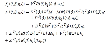
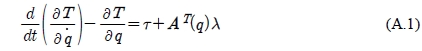
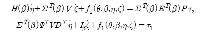
Applying the well known Lagrange equation to the motion of the AGV with nonholonomic constraints, the dynamic equation for the AGV can be obtained as follows [Appendix]:
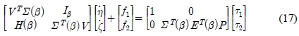
where f1 and f2 are scalar functions depending on θ, β, η and ζ.

τ1 and τ2 are the torques applied to the steering wheel for its orientation and rotation, respectively.
Equation (17) can be rewritten as follows:
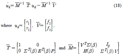
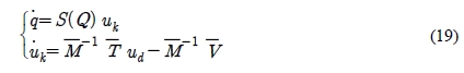
From Equation (13) and Equation (18), the final system equations are given as follows:
3. Measurement of Tracking Errors using Camera Sensor
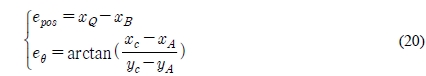
Figure 2 shows schematic for the tracking errors of AGV. epos is the position error between the position of the tracking point Q on the AGV and the reference point on the reference path. eθ is the angle error between the YQ axis and the tangent line of the path at the reference point.

Schematic for the tracking errors of AGV
Figure 3 shows the schematic of camera window for measuring the tracking errors using camera sensor. The camera sensor is a Logitech webcam C600. The webcam specification is up to 30 frames per second, 2.0-megapixel sensor and hi-speed USB 2.0 communication. The camera has a resolution of 640pixel × 480pixel

Schematic for measuring the tracking errors using camera sensor
The camera window is fixed on camera and captures the images of 15cm × 15cm. The image size is small in comparison with curvature radius of the reference path. Therefore, it is assumed that the image of reference path is straight line as shown in Figure 3.

Image processing procedure
Form Figure 3, the tracking errors can be obtained as follows:
Images captured from web camera are processed by using AForge, NET framework, C# framework designed for developers and researchers in the fields of computer vision and artificial intelligence. To calculate the position error and the angle error from the image captured by camera, image processing procedure includes steps a shown as follows:
4. Controller Design
To control the AGV for path following, a control algorithm is designed as in Figure 5. The controller integrates two control loops, kinematic control loop based on fuzzy logic framework and dynamic control loop based on two conventional PID controllers.

Structure of the proposed path-following controller for AGV
The fuzzy controller uses the tracking error vector as its inputs including the position error, the angle error and the derivative of angle error. The fuzzy outputs are derivative of the linear velocity, and the angular velocity at the tracking point, Q.
From the fuzzy output, the velocity control vector at the tracking point is achieved. Because the AGV is driven by the steering driving wheel, the steering angle and the angular velocity of the steering wheel should be calculated. Finally, in dynamic control loop, two PID controllers are used to control two DC motors for tracking the desired steering angle and angular velocity of the steering wheel.
4.1 Fuzzy controller Design
Fuzzy rules are normally created based on human experience and logic. Therefore, it is necessary to analyze the desired outputs based on available inputs. From two inputs, the position error and the angle error, AGV posture is defined in 9 different situations as shown in Figure 6. From 9 situations, 9 rules are generated, respectively. In addition, two other rules are proposed when derivative of angle error are large, especially while the robot moves away the path with high velocity.

Structure of a fuzzy controller
Table 1 shows the fuzzy rules designed for AGV for path following and the membership functions are given in Figure 7.

Fuzzy rules

Membership functions
4.2 PID controller Design
The dynamic control loop includes two PID controllers in Figure 8. The first one is used for tracking the desired steering angle, βd.

Dynamic control loop
The second one is used for tracking the desired rotation angular velocity of steering wheel, ηd.
A PID controller 1 is designed based on steering angle error of the steering wheel as follows:
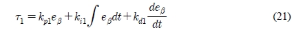

where kp1, ki1 and kd1 are the coefficients of the PID controller 1.
A PID controller 2 is designed based on rotational angular velocity error as follows:
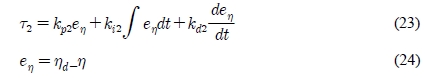
where kp2, ki2 and kd2 are the coefficients of the PID controller 2.
5. Simulation and Experimental Results
To verify the effectiveness of the proposed controllers, simulations and experiments have been done for the AGV to follow an unknown path. In the simulation, the initial values and the numerical parameter values are given in Table 2 and Table 3.
Initial values for simulation
Numerical parameter values of AGV
The reference path has five segments with three straight line segments and two curved line segments. The radius of the first curve is 6 m and the radius of the second curve is 4 m. Figure 9 shows the reference path in simulations and experiments.

Reference path
The coefficients in two PID controllers are obtained by trial and error method in simulations and experiments. Their numerical values are given as follows: kp1 = 300, ki1 = 0.5, kd1 = 25, kp2 = 200, ki2 = 5, kd2 =5. Figure 10 shows the position error that becomes zero when the path is a straight line and is bounded within ± 0.1m in both simulation and experimental results when the path is a curved line. Figure 11 shows angle error that is bounded within ± 0.8o in both simulation and experimental results. Figure 12 shows steering angle of steering wheel in experiment and the steering wheel angle is bounded within 90o ± 40o in both simulation and experimental results. Figure 13 shows the linear velocity of AGV at tracking point Q
The linear velocity is limited within 0.5m/s and 2m/s in both simulation and experimental results. Figure 14 shows the path following result of the AGV in experiment.

Position error

Angle error

Steering angle of steering wheel

Linear velocity of tracking point on AGV

Path following result of the AGV in experiment
6. Conclusions
This paper developed an industrial AGV, a tricycle wheeled mobile robot. First, kinematic model and dynamic model of the AGV were presented. Second, schematic of tracking errors using camera sensor were defined. After that, control algorithm for path-following of AGV was proposed based on integration of two control loops, kinematic control loop and dynamic control loop. The kinematic control loop based on fuzzy logic framework and the dynamic control loop based on two PID controllers were designed. The effectiveness of the proposed system was shown through simulation and experimental results. The AGV could follow the desired path with a large enough curvature radius smoothly. So the system could be applied and implemented to the industrial field in practical.
Acknowledgments
This research was supported by a grant of preparatory association from Pukyong National University.
This paper is extended and updated from the short version that appeared in the Proceedings of the International symposium on Marine Engineering and Technology (ISMT 2014), held at Paradise Hotel, Busan, Korea on September 17-19, 2014.
References
-
V. T. Dinh, P. T. Doan, G. Hoang, H. K. Kim, S. J. Oh, and S. B. Kim, “Motion control of an omnidirectional mobile platform for path following using backstepping technique”, Journal of Ocean Engineering and Technology, 25(5), p1-8, (2011).
[https://doi.org/10.5574/KSOE.2011.25.5.001]

-
N. Hung, V. T. Dinh, J. S. Im, H. K. Kim, and S. B. Kim, “Motion control of an omnidirectional mobile platform for trajectory tracking using an integral sliding mode controller”, International Journal of Control, Automation and Systems, 8(6), p1221-1231, (2010).
[https://doi.org/10.1007/s12555-010-0607-8]
-
T. L. Bui, P. T. Doan, H. K. Kim, V. G. Nguyen, and S. B. Kim, “Adaptive motion controller design for an omnidirectional AGV based on laser sensor”, Journal of AETA 2013: Recent Advances in Electrical Engineering and Related Sciences, 282, p509-523, (2014).
[https://doi.org/10.1007/978-3-642-41968-3_51]
-
M Eghtesad, and D. S. Necsulescu, “Experimental study of the dynamic based feedback linearization of an autonomous wheeled ground vehicle”, Journal of Robotics and Autonomous Systems, 47, p47-63, (2004).
[https://doi.org/10.1016/j.robot.2004.02.003]
-
E. Aguirre, and A. Gonzàlez, “Fuzzy behaviors for mobile robot navigation : design, coordination and fusion”, International Journal of Approximate Reasoning, 25, p255-289, (2000).
[https://doi.org/10.1016/S0888-613X(00)00056-6]
-
H. Maaref, and C. Barret, “Sensor-based fuzzy navigation of an autonomous mobile robot in an indoor environment”, Journal of Control Engineering Practice, 8, p757-768, July), (2000.
[https://doi.org/10.1016/S0967-0661(99)00200-2]
-
I. Baturone, F. Moreno-Velo, S. Sànchez-Solano, and A. Ollero, “Automatic design of fuzzy controllers for car-like autonomous robots”, IEEE Transactions on Fuzzy Systems, 12(4), p447-465, (2004).
[https://doi.org/10.1109/TFUZZ.2004.832532]
-
H. Li, and S. J. Chang, “Autonomous fuzzy parking control of a car-like mobile robots”, IEEE Transaction on System, Man, Cybernetics-Part A, Systems and Humans, 33(4), p451-465, (2003).
[https://doi.org/10.1109/TSMCA.2003.811766]
-
T. H. Li, S. J. Chang, and Y. X. Chen, “Implementation of human like driving skills by autonomous fuzzy behavior control on an FPGA based car-Like mobile robot”, IEEE Transactions on Industrial Electronics, 50, p867-880, (2003).
[https://doi.org/10.1109/TIE.2003.817490]
-
O. Sánchez, A. Ollero, and G. Heredia, “Adaptive fuzzy control for automatic path tracking of outdoor mobile robots. Application to Romeo 3r”, Proceedings of the 6th International Conference Fuzzy Systems, Barcelona, p593-599, (1997).
[https://doi.org/10.1109/FUZZY.1997.616433]
-
R. Precup, S. Preitl, and Z. Preitl, “Fuzzy control solution for a class of tricycle mobile robots”, Proceedings of the 2006 IEEE International Conference on Mechatronics, p203-208, (2006).
[https://doi.org/10.1109/ICMECH.2006.252525]
-
G. Antonelli, S. Chiaverini, and G. Fusco, “A fuzzy-logic-based approach for mobile robot path tracking”, IEEE Transaction on Fuzzy Systems, 15(2), p211-221, (2007).
[https://doi.org/10.1109/TFUZZ.2006.879998]
- C. Juang, and C. Hsu, “Reinforcement ant optimized fuzzy controller for mobile-robot wall-following control”, IEEE Transaction on Industrial Electronics, 56(10), p3931-3940, (2009).
- N. Liu, “Intelligent path following method for non-holonomic robot using fuzzy control”, 2009 Second International Conference on Intelligent Networks and Intelligent Systems, p282-285, (2009).
- C. Juang, and Y. Chang, “Evolutionary - group - based particle -swam - optimized fuzzy controller with application to mobile-robot navigation in unknown environments”, IEEE Transactions on Fuzzy System, 19(2), (2011).
-
I. Baturone, F. J. Moreno, V. Blanco, and J. Ferruz, “Design of embedded DSP-based fuzzy controllers for autonomous mobile robots”, IEEE Transaction on Industrial Electronics, 55(2), p928-936, (2008).
[https://doi.org/10.1109/TIE.2007.896547]
-
Y. H. Lee, G. G. Jin, and M.O. So, “Level control of single water tank systems using Fuzzy-PID technique”, Journal of the Korean Society of Marine Engineering, 38(5), p550-556, (2014).
[https://doi.org/10.5916/jkosme.2014.38.5.550]
-
G. Campion, G. Bastin, B. D. Andreá-Novel, “Structural properties and classification of kinematic and dynamic models of wheeled mobile robots”, IEEE Transactions on Robotics and Automation, 12(1), p47-62, (1996).
[https://doi.org/10.1109/70.481750]
- L. Gracia, and J. Tornero, “Kinematic control of wheeled mobile robots”, Latin American Applied Research, 38, p7-16, (2008).
-
A. Kamga, A. Rachid, “Speed, steering angle and path tracking controls for a tricycle robot”, Proceedings of the 1996 IEEE International Symposium on Computer-Aided Control System Design, Dearborn, MI, p56-56, (1996).
[https://doi.org/10.1109/CACSD.1996.555197]
Appendix
Lagrange equation for nonholonomic constraints to the motion of the AGV as follows:
The following compact notation is defined.
By separating q into three components, ξ , β and Φ , the following equations are obtained.
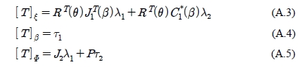
where λ1 = [λ1 λ2 λ3]Τ and λ2 = [λ21 λ222]Τ are the Lagrange multipliers vectors associated with the constrains Equation (6) and Equation (8), respectively.
By eliminating the Lagrange multipliers from Equation (A.3) and Equation (A.5), the following are obtained.

Substituting Τ from Equation (16) to Equation (A.1) can be obtained as the following:
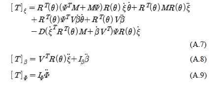
From the kinematic Equation (5), Equation (11) and Equation (12), the following are obtained.
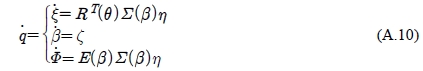
Derivatives of
 is obtained as follows:
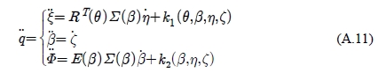
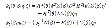
where k1 and k2 are 3 × 1 vectors depending on θ, β, η and ζ.
Using Equation (A.10) and Equation (A.11), eliminating the velocities
 and the acceleration
 in (A.4) and (A.6) yields:
where f1 and f2 are scalar functions depending on θ, β, η and ζ.