CO concentration distribution in a tunnel model closed at left end side using CFD

1. Introduction

Carbon monoxide (CO) is one of the classical pollutants that have set air quality limit values in many countries. CO is chosen as an indicator of air quality to assist the design of tunnel ventilation systems [1]. Significant sources of CO are resulted from incomplete combustion of hydrocarbon fuels and tobacco smoking. McQuiston et al. [2] mentioned that carbon monoxide levels near 15 ppm are harmful and can significantly affect body chemistry. The reaction of humans to different CO levels varies significantly, and the effects can be cumulative. CO is not only a potentially lethal air pollutant in itself, but also a precursor for other pollutants.

Stochastic Box-Jenkins models [3] were used to forecast carbon monoxide concentration levels of various pollutants by applying time-series analysis by statistical means. Chelani and Devotta [4] attempted to assess the predictability of CO concentration in an urban area using nonlinear dynamical system theory. To determine the extent of real-time prediction of extreme ambient CO concentrations, Sharma and Khare [5] used univariate linear stochastic models based on the Box-Jenkins modelling techniques. Abbasloo et al. [1] obtained three dimensional CO concentration distribution in a two-way underground tunnel using standard k-ε turbulence model. To validate the model and the concepts, the concentration of CO was experimentally measured as well. Zhang and Batterman [6] contrasted simulation and statistical models to estimate traffic impacts on CO and PM_2.5 concentrations near highways. Air pollutant concentrations of CO and particle matter less than 2.5 μm in diameter have been considered.

According to the increasing number of tunnel structures in general transportation systems, a special interest in safety regarding polluted air has significantly grown. Focused on smoke control for fire safety in those various tunnels, many investigations have been carried out [7][10].

There are three types of tunnels, which are closed at both end sides, closed at one end side, and opened at both end sides. In case of a coal mine, one tunnel end is closed, whereas the other is open. The influence of ventilation tube rupture in a coal mine tunnel was investigated by Kun et al. [11]. Flow characteristics regarding velocity vector fields, pressure distributions, turbulence kinetic energy in the tunnel models opened and closed at both end sides are discussed using CFD [12]. Through the PIV system based on the reliable field measurement technique in tunnel models, velocity maps, vorticity maps, and kinetic energy distributions are investigated [13].

This study is particularly focused on the distributions of the CO concentrations in the tunnel model closed at left end side. It is aimed at providing reliable predictions of CO concentration distributions in the tunnel model using the ANSYS CFX as a commercial CFD code. The CO gas flow with no heat source entrained into the model through the inlet is considered at three different Reynolds numbers. The CO concentrations in connection with flow velocity and pressure distributions are useful to provide some desirable information in determining the better ventilation system in the tunnel model closed at the left end side alone.

2. Physical Model

Figure 1 shows the computational grids of the tunnel model closed at the left end side alone. The tunnel model is 800 mm long and the dimension of the square cross section is 80 mm × 80 mm. In order to analyze the flow characteristics in the previous experimental paper [13] using PIV system, a 800 mm long tunnel model, which is reduced to 1/100 of its actual length, is used on the basis of the similarity laws of fluid flow.

Figure 1:

Computational grids of the three tunnel models

The CO gas flow entering the tunnel model from the inlet is assumed to be steady, and the walls inside the tunnel model are supposed to be adiabatic. The kinematic viscosity of the CO gas entering the model through the inlet is 13.28 × 10^-6 m²/s. The inlet flow velocities are given at 0.3, 0.6, and 1.0 m/s in order to analyze the computational CO concentrations in terms of the three different Reynolds numbers. ANSYS CFX, which is a commercial CFD program, has been implemented. To investigate the effective viscosity at low Reynolds numbers, the Re-Normalization Group (RNG) k-ε model is used for predicting indoor concentration distributions effectively in three different tunnel models.

Figure 2:

Computational mesh near the walls

Figure 2 shows the computational mesh for the cross section of the model to be generated by ANSYS ICEM CFD as a grid generation tool. Around 300,000 quadrilateral grids are meshed to properly resolve the viscous-affected region near the tunnel walls. By using an excessively fine mesh near the walls, the validity of near-wall modeling is extended. No-slip conditions are imposed on all sides of the walls inside the models.

Figure 3:

CO concentration points measured using CFD

Five points of A, B, C, D, and E are given as shown in Figure 3 to numerically obtain carbon monoxide concentrations using CFD. The length to height ratio, x/H, is defined as the ratio of measuring distance from the inlet centerline to the tunnel height. The ratio means the position where CO concentrations are measured numerically as using CFD. Each point from A to E corresponds to x/H of -5.0, -2.5, 0, +2.5, and +5.0, respectively. The inlet of the tunnel model, which is located at the middle of the tunnel floor in the x-z plane, has a cross sectional area of 30mm × 80mm, whereas the outlet having the same area of the inlet is located on the ceiling of the tunnel model at L=+60mm, where L is defined as a distance from the vertical centerline of the inlet in the x-direction.

3. Results and Discussion

The CO concentrations are investigated in terms of three different Reynolds numbers inside the tunnel model, which is closed at the left end side and opened at the right. The three Reynolds numbers caused by the inlet velocities, at which CO gas flows into the model through the inlet on the tunnel floor, are 990, 1970, and 3200, respectively. The outlet on the tunnel ceiling is located at x/H=+0.75 away from the inlet centerline. The flow characteristics due to the distributions of the CO concentration inside the tunnel model closed at the left end side alone are discussed below. Carbon monoxide concentrations in this paper are expressed as the volume fraction defined as the volume of CO gas divided by the volume of the ambient air inside the tunnel model. In order to obtain and analyze the CO concentrations, five points in the x-y plane are chosen at the tunnel height of 40mm, 0.5H, over the longitudinal centerline of the tunnel floor.

3.1 CO Concentrations inside the Tunnel Model Closed at Left End Side Alone over Time

In Figure 4 (a), the CO concentrations at x/H=-5.0 and -2.5 simultaneously increase in the similar way that those in the case of the tunnel model closed at both end sides do [14]. In addition, the level of CO concentrations is also very similar to that of the closed model case. However, the CO concentrations at x/H=0 and +2.5 already approach a volume fraction of 0.99 at ten seconds. While at x/H=+5.0, its concentration is 0.25 at ten seconds and also reaches 0.99 just after twenty seconds. It is observed that the concentration changes of x/H=-5.0 and -2.5 have the similar characteristics like the case of the tunnel model closed at both end sides, and its concentration at x/H=0 with a volume fraction of 0.99 is directly affected by the outlet.

Figure 4 (b) illustrates the CO volume fraction concentrations with time at a Reynolds number of 1970. The CO concentration curves at x/H=-5.0 and -2.5 go up lower than those at Re=990, and also in this case the curves are formed in pairs, similar to those at Re=990. It is inferred that in these two cases for lower Reynolds number, the CO flows near the closed tunnel region on the left side show the laminar characteristics. The CO concentration at x/H=0, where the measured point is closer to the outlet of the model, remains almost unchanged with a volume fraction of 0.97, regardless of the model tunnel closed or opened at end sides. At x/H=+2.5, the concentrations are changed from 0.61 to 0.88 over time. At x/H=+5.0, where the point is open at the end side, the concentration reaches 0.96 at ten seconds and then keeps 0.99 after twenty seconds.

Figure 4:

CO concentration levels at given distances from the inlet centerline with time in the tunnel model closed at left end side(a) CO concentration at Re=990

(b) CO concentration at Re=1970

(c) CO concentration at Re=3290

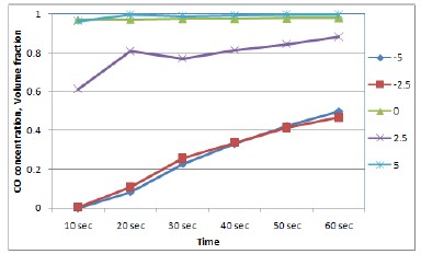
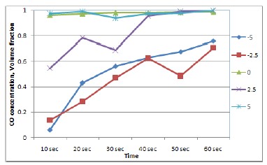
Figure 4 (c) depicts the variations of CO concentrations with time at a Reynolds number of 3290. The increase in Reynolds number at x/H=-5.0 and -2.5 is accompanied by a bigger increase in the CO concentration, when compared to the case of Re=1970. Once again, as the Reynolds number increases, the CO concentrations irregularly increase inside the tunnel model except for both x/H=0 and +5.0. At x/H=+2.5, the volume fraction of CO gas goes up 0.96 in forty seconds, similar to those at x/H=0 and +5.0.

3.2 Comparison of CO Concentrations in terms of Two Different Measuring Times

To get deeper information about the CO concentration distributions in the tunnel model at ten and sixty seconds after the beginning of the simulation, contour plots of CO concentrations are shown in Figures 5 and 6. For each case in the figures below, the first contours depending on the Reynolds number depict the CO concentrations in the x-y vertical plane and the second ones do in the x-z horizontal plane at 0.5H. The left half of the contours is called the negative x-direction, while the other right half is done the positive x-direction.

3.2.1 CO concentrations in 10 seconds

Figure 5:

Contour plots of CO concentrations at three different Reynolds numbers in ten seconds(a) CO concentrations at Re=990

(b) CO concentrations at Re=1970

(c) CO concentrations at Re=3290

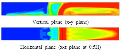
As shown in Figure 5 (a), the CO concentrations in the positive x-direction from the inlet centerline and expecially in the vicinity of the outlet are much higher than those in the negative x-direction. At the upper right corner of the tunnel model opened at the right end side in the positive x-direction, not in the negative x-direction, are lower concentrations than in its surroundings inside the tunnel. It can be inferred that the concentrations are changed slowly and widely due to the very low Reynolds number of 990.

At Re=1970, the diffusion velocity of CO concentration is faster from the inlet to the outlet than that of Re=990 in the positive x-direction in Figure 5 (b). The size of rising CO concentration in the adjacent field of the inlet is more widely extended compared to that of Re=990. In the central x-z horizontal plane, the CO concentrations on the central axis are longitudinally symmetrical. The concentrations in the negative x-direction in the horizontal plane are generally constant, but those in the central region in the positive x-direction are lower than those near the both walls in the tunnel.

At Re=3290, as shown in Figure 5 (c) on the negative vertical plane, the size of rising CO concentrations has doubled compared to that of R=1970 as well. The distributions of the highest CO concentrations from the inlet to the ceiling are more tilted to the positive x-direction than those at Re=1970. However, the CO concentrations on the horizontal plane in the positive x-direction from the inlet centerline are becoming lower than those in the cases of Re=990 and 1290. It can not be mentioned therefore that, even though in ten seconds the Reynolds number increases, the CO concentrations on the x-z plane in the positive x-direction do always increase all together inside the tunnel.

3.2.2 CO concentrations in 60 seconds

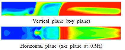
Figure 6 (a) shows the contours of CO concentrations in sixty seconds at Re= 990. The CO concentrations of the upper part near the tunnel ceiling in the negative x-direction keep very low, even though it takes fifty seconds after the first ten seconds of measuring the CO movements. The scope of the higher CO concentration, although limited near the bottom region within ten seconds, is much more extended upward in sixty seconds.

In the positive x-direction, the CO concentration levels remain very high throughout the whole region, except for an elliptical-shaped region below the centerline between x/H=+1.4 and +2.8. The concentration levels in the x-z plane at 0.5H are divided into two zones on the basis of the inlet centerline. The lower concentration zone is formed on the left side of the inlet and the higher one is on the right. Each of the concentration levels in both regions is very constant due to a very low Reynolds number of 990.

Figure 6:

Contour plots of CO concentrations at three different Reynolds numbers in sixty seconds(a) CO concentrations at Re=990

(b) CO concentrations at Re=1970

(c) CO concentrations at Re=3290

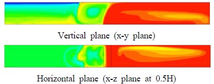
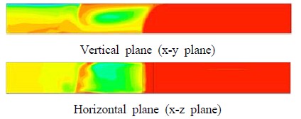
Figure 6 (b) shows the CO concentrations at Re=1970 in sixty seconds. The region, in which the concentration is very low near the tunnel ceiling in the negative x-direction, is considerably scaled down when compared to that of Re=990. In the negative x-z horizontal plane, the CO concentration with the volume fraction of 0.47 at Re=1970 is some lower than that of 0.68 at Re=990. It can be observed that any vortex is formed on the left side of the inlet centerline due to the increased inlet velocity. Although the concentration is very high through the tunnel in the positive x-direction relatively a little lower concentrations are distributed widely in the middle region of the tunnel between the inlet and the open end side.

Figure 6 (c) shows the distributions of transient CO concentration in sixty second at a Reynolds number of 3290. The concentration levels near the ceiling in the negative x-direction still remain a little lower, yet have increased throughout the tunnel when compared to those of Re=990 and 1290. The vortex formation, which is obviously elliptic-shaped, is observed on the left side of the inlet centerline.

The vortex on the horizontal plane in the negative x-direction near the inlet centerline is shown in the shape of a rectangle. From x/H=0 to x/H=+5.0, most of the concentration levels are very high regardless of any positions inside the tunnel.

Table 1:

CO volume fractions predicted at five central positions in 10 and 60 seconds, depending on the three Reynolds numbers(a) 10 seconds after the start of the simulation

(b) 60 seconds after the start of the simulation

To analyze the change of average CO concentrations at three different Reynolds numbers, CO volume fractions predicted at five central positions in terms of two observed times are listed in Table 1. The average concentrations of CO in ten seconds are increased as the Reynolds number increases, as presented in Table 1 (a). On the other hand, the average concentration in sixty seconds for Re=1970 decreases by about 10.8 percents, compared to that for Re=990, as presented in Table 1 (b). It can be seen that, though the inlet velocity increases, the average CO concentrations in a very short time don't necessarily increase.

During the time interval of fifty seconds from ten to sixty seconds, each of the average CO concentrations at three different Reynolds numbers increases by 35.3 percent at Re=990, 40.7 at Re=1970, and 25.4 at Re=3290, respectively. The total average of CO concentrations inside the tunnel model increases by 50.3 percent at ten seconds after the start of the simulation, and relatively does 33.8 percent after sixty seconds, compared to those in ten seconds.

3.2.3 Average CO concentration variations in three different models

Figure 7:

Averaged variations of carbon monoxide concentration predicted in three different tunnel models depending on three Reynolds numbers.

Considerable variations in CO concentration at three different Reynolds numbers are predicted according to three different tunnel models: 1) tunnel closed at both end sides, 2) tunnel closed at left end side alone, and 3) tunnel opened at both end sides. In Figure 7, these concentration data here applied to the tunnel models closed and opened at both end sides come from the previous paper [14]. Regarding the three different tunnel models in the order in which they are shown in Figure 7, each of averaged CO concentrations between ten seconds to sixty seconds after the start of the simulation increases 155.6, 67.2 and 10.1 percents respectively, when based on each of the models at ten seconds. During the fifty seconds, the largest variations in CO concentration appear in case of the model closed at both end sides, as expected before. On the other hand, there is just a little change of CO concentrations in case of the model opened at both end sides even though average CO concentration levels are very high.

At Re=1970 when compared to Re=990 and 3290 in sixty seconds, relatively lower average CO concentration variations are shown in case of the closed and the half closed models, while some exceptional concentration variations are indicated in case of the tunnel model opened at both end sides. These irregular CO concentration variations at Re=1790 are considered that the transition from laminar to turbulent flow occurs even in three different tunnel models. It can be seen that the average concentration variations are related with time depending on the type of tunnel models and the different Reynolds numbers.

4. Conclusions

Carbon Monoxide (CO), which is an odorless and colorless gas formed in the process of incomplete combustion of fuel in power generators, is dangerous because it interferes with normal oxygen uptake for humans. To support the exploration and analysis of results from CFD simulation, the visualization approach of time-dependent data is effectively used to predict the CO concentration distributions in this paper. The CFD results from the tunnel model closed at one end side are the following:

(1) At Re=1970 when compared to Re=990 and 3290 in sixty seconds, relatively lower average CO concentration variations are shown in case of the tunnel models closed at both end sides and closed at one end side, while some exceptional concentration variations are indicated in case of the tunnel model opened at both end sides. These irregular CO concentration variations at Re=1790 are considered that transitional flows are dominant even in three different tunnel models.

(2) The CO concentration at x/H=0, where the measured point is closer to the outlet of the model, remains almost unchanged with a volume fraction of 0.97, regardless of the model tunnel closed or opened at the end sides.

(3) The total average of CO concentrations inside the tunnel model increases by 50.3 percent at ten seconds after the start of the simulation, and relatively does 33.8 percent after sixty seconds, compared to those after ten seconds.

(4) The average concentrations of CO are increased as the Reynolds number increases. On the other hand, the average concentration after sixty seconds for Re=1970 decreases by about 10.8 percents, compared to that for Re=990. It can be seen that, though the inlet velocity increases, the average CO concentrations in a very short time don't necessarily increase.

References

• A. Abbasloo, J. F. Kaljahi, and F. Esmaeilzadeh, “Prediction of three dimensional CO concentration distribution in zand tunnel of shiraz using computational fluid dynamic method”, Journal of Applied Environmental and Biological Sciences, 2(1), p67-76, (2012).
• F. C. McQuiston, J. D. Parker, and J. D. Spitler, Heating, Ventilating, and Air Conditioning: Analysis and Design, 6/e, John Wiley & Sons, Inc, (2005).
• G. E. P. Box, Time Series Analysis, Forecasting and Control, Holden-Days, San Francisco, (1970).
• A. B. Chelani, and S. Devotta, “Prediction of ambient carbon monoxide concentration using nonlinear time series analysis technique”, Transportation Research Part D 12, p569-600, (2007).
• P. Sharma, and M. Khare, “Real-time prediction of extreme ambient carbon monoxide concentrations due to vehicular exhaust emissions using univariate linear stochastic models”, Transportation Research Part D 5, p59-69, (2000). [https://doi.org/10.1016/S1361-9209(99)00024-3]
• K. Zhang, and S. Batterman, “Near-road air pollutant concentrations of CO and PM_2.5: A comparison of MOBILE6.2/CALINE4 and generalized additive models”, Atmosphere Environment, 44, p1740-1748, (2010). [https://doi.org/10.1016/j.atmosenv.2010.02.008]
• Olivier Vauquelin, “Experimental simulations of fire-induced smoke control in tunnels using an 'air-helium reduced scale model' : Principle, limitations, results and future”, Tunnelling and Underground space Technology, 23, p171-178, (2008). [https://doi.org/10.1016/j.tust.2007.04.003]
• C. C. Hwang, J. C. Edwards, “The critical ventilation velocity in tunnel fires - a computer simulation”, Fire Safety Journal, 40, p213-244, (2005). [https://doi.org/10.1016/j.firesaf.2004.11.001]
• C. C. Hwang, J. D. Wargo, “Experimental study of thermally generated reverse stratified layers in a fire tunnel”, Combust Flame, 66, p171-80, (1986). [https://doi.org/10.1016/0010-2180(86)90089-1]
• Y Wu, and Baker, M. Z. A, “Control of smoke flow in tunnel fires using longitudinal ventilation systems - a study of the critical velocity”, Fire Safety Journal, 35, p363-390, (2000). [https://doi.org/10.1016/S0379-7112(00)00031-X]
• Li, Kun, Ding, Cui, You, Chang-fu, “Influence of ventilation tube rupture from fires on secondary catastrophes in tunnel”, First international symposium on mine safety science and engineering, Procedia Engineering, 26, p75-83, (2011). [https://doi.org/10.1016/j.proeng.2011.11.2142]
• Y.-H. Lee, “Flow behavior in a rectangular tunnel opened and closed at both sides using CFD”, Journal of the Korean Society of Marine Engineering, 36(3), p368-377, (2012). [https://doi.org/10.5916/jkosme.2012.36.3.368]
• Y.-H. Lee, “Experimental and CFD simulations of polluted air behavior in rectangular tunnels”, Journal of the Korean society of marin engineering, 35(5), p608-615, (2011), (in Korean). [https://doi.org/10.5916/jkosme.2011.35.5.608]
• Y.-H Lee, “Distribution of CO concentration in two tunnel models using CFD”, Journal of the Korean Society of Marine Engineering, 36(7), p910-918, (2012). [https://doi.org/10.5916/jkosme.2012.36.7.910]