A fundamental study on velocity restoration for tidal farm

2.1 Actuator disc theory

Albert Betz (1885 - 1968), a German physicist and a pioneer of wind turbine technology, introduced a method to determine the limit power of extraction in a fluid. That is the "Actuator Disc Theory", the method [3] for characterization of an actual tidal turbine in a solution of Reynolds-averaged Navier-Stokes equations. The application of the model in an infinite volume of air is used in the analysis and design of wind turbines. Since the flow of air in the atmosphere is different to that of a liquid constrained in an open channel due to the air's negligible density, actuator disc theory can be applied for tidal turbines with some modification and extra consideration. Actuator disc play an important role in study of multi turbine array. Thus, the flow field including turbines becomes a huge domain, a so-called tidal farm. It can be very convenient technically and economically if a whole turbine farm is simulated by means of actuator disc theory.

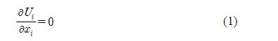
The true fluid flow passing around and through a tidal turbine is governed by the Reynolds-averaged Navier-Stokes (RANS) equations. They are timeaveraged equations of motion for fluid flow. Thus, combining the law of conservation of mass with the transport theorem yields the continuity equation and is written as:

The momentum equation expresses Newton's second law of motion for a fluid flowing through a finite control volume. This study is steady state analysis, so the equation is:

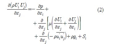
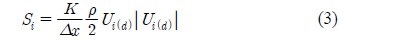
Reynolds stress is resolved by turbulence model. Si represents the immersing effect of turbine at disc region and is calculated as follow:

Figure 1:

Actuator disc demonstration

Resistance coefficient of turbine is found to be 2 for most practical case [4]. K = 0 corresponds to free flow state, or no turbine is submerged into the stream. K = 4 corresponds to break-state, meaning turbine is unable to rotate or no water passes through the disc.

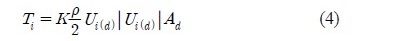
The actuator disc is applied a constant resistance to the incoming flow. This resistance causes a thrust to be imposed on the flow and this thrust should be similar to that imposed by the turbine simulated. For a turbine, thrust will vary based on the incoming flow, geometry, pitch of the blades, and rotational speed. For an actuator disc, thrust depends on its resistance coefficient and the inflow velocity, this is shown as:

The turbine is then typically characterized in terms of its thrust coefficient, which is defined as:

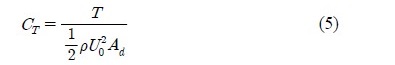
By characterizing an actuator disc with a given CT which features a real turbine's characteristic, the disc becomes a represented tidal turbine. Therefore, results from actuator disc simulation can be used to evaluate real turbine's performance with acceptable accuracy [2].

2.2 Calculation conditions

Initial input parameters are listed in Table 1. This calculation domain is made for a scale scenario with Froude number, Fr = 0.175. Thus, it is corresponded to an actual model of 10m turbine in a 30m water depth channel with mean inflow velocity of 3m/s. Typical value of Froude number for full scale channels are within 0.1 - 0.2, and value less than 0.5 generally ensure stable flow when there are no obstacles in water column [5].

Boundary conditions are as follows:

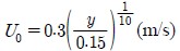
Inlet: Cartesian normal speed. Since the flow is affected by seabed surface roughness, the velocity has gradient characteristic as defined by 1/10th power law. Initial water level is set to 0.3m.

Outlet: Static pressure.

Sidewall: Free slip wall boundary.

Bed plane: As real sea bed is rough surface. So nonslip wall is defined for this boundary.

Disc front and rear walls: Free slip walls with flux sources.

Disc cylinder: Free slip wall.

Free surface: Volume of fluid model [6][7].

Simulation using ANSYS CFX [8] is done in steady state. Turbulence model k-ε is used since it is the most commonly used of all the turbulence models in CFD [9]. For steady state calculations, max integration is set to 4,000 to ensure convergence with convergence criteria of 1×10^-5.

The axial induction (sometimes called interference) factor, a, is defined as the fractional decrease in wind velocity between the free stream (upwind) and the rotor plane:

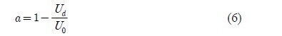
As a increases from zero, the downwind flow speed steadily decreases until, a = 1/2, meaning that the rotor has completely stopped and the simple theory is no longer applicable. According to Betz theory, turbine reaches maximum power efficiency at a = 1/3, corresponds to C_T = 0.89 [10].

Table 1

Initial calculation conditions

3.1 Lateral turbine array

The previous section stated that the longitudinal spacing has major influence to turbine. Turbines in tidal farm are also positioned laterally, so the influence of lateral spacing should as well be evaluated. However, since the lateral array turbines do not share the same inline stream, the lateral spacing is much shorter than longitudinal spacing. Lateral spacing is set just to avoid disturbance effect of turbines due to their downstream wakes.

The calculation domain for lateral positioned turbine array adopted hexa mesh style which consists of one million nodes (Figure 2). The domain is shown in Figure 3. Simulation is done for three cases corresponding to three different lateral spacings: 2.0D, 2.5D and 3.0D. Domain size is 8m(L)×1m(W)×0.5m(H) which is large enough to position three discs inline along the width in all cases.

Figure 2:

Mesh formation of lateral array

In this simulation, turbines are numbered No. 1, No. 2 and No. 3 from left to right as marked in Figure 3.

Figure 3:

Calculation domain of lateral array

Flow visualization in horizontal view (XY plane) is shown in Figure 4. According to the flow pattern, three cases show the similar velocity contours of water and air. In 3D lateral spacing case, there is a small fluctuation of air velocity at inlet, but this is not considered as an influence to the turbine group's performance since there is no abnormal variation in water velocity. These contours generally present the flow pattern in term of visualization.

Figure 5 shows the velocity deficit along the centerline of turbines at different lateral spacings. For 2D lateral spacing, turbine No. 2 obtains the highest power coefficient, C_P2 = 49.48%, the two remaining have the same lower value, C_P1 = C_P3 = 49.23%. Since turbine No. 2 absorbed more power, its restoration is slower than the rest (Fig. 5a), but all of them show the similar restoration characteristic at far wake location, from 60D to 70D. Maximum restoration reaches 96% at 70D downstream location.

Figure 4:

Mesh formation of lateral array

When the lateral spacing is increased to 2.5D, the three turbines get their power coefficients C_P1 = 49.25%, C_P2 = 49.48% and C_P3 = 49.33%, respectively. The difference in power efficiency is relatively reduced but clarified deficit of the three turbines is still visible in Fig. 5b. The restoration of the three is almost the same and also reaches 96% at 70D.

When the lateral spacing is increased to 3D, all three turbines almost have the same deficit curve. Their power coefficients all reach 49.48%.Thus, these results show that 3D lateral spacing is wide enough to minimum mutual influence between the lateral array turbines. And in this arrangement, fully restoration is visible at 70D downstream location. But in fact, it is uneconomical to arrange turbine array with longitudinal spacing up to 70D. Instead, the range from 20D to 30D in previous study is claimed to be long enough for longitudinal spacing, with thin this value high restoration rate of about 80-90% is available and acceptable. Therefore, more spacing is saved for other arrays.

Figure 5:

Deficit along the centerline in lateral array

Thus, according to these results, all cases are selectable since the lateral influence is not as considerable as compared to longitudinal case. 3D is found to be the optimum lateral spacing in current study but 2.0D will be more advantageous in narrow channels.

3.2 Staggered turbine array

Staggered formation is a well known formation in which elements are at different levels and are not abreast of each other. This is to ensure the safe interaction among elements in some group operation. Staggered formation can be applied to tidal turbine farm and it is claimed as an effective formation for the longterm stable operation of tidal turbines.

Previous study has shown that 3D lateral spacing and 20D-35D longitudinal spacing are enough to ensure the stable operation of turbines and minimum the disturbance effects between them [2]. Thus, these settings are applied in staggered formation simulation. In detail, the number of turbine is chosen to be seven, they will be spaced 30D longitudinally and 3D laterally. The turbine group is positioned in staggered formation as shown in Fig. 6 which shows the calculation domain; turbines are numbered from 1 to 7. Figure 7 shows the mesh formation for this domain. The mesh contains 1 million nodes, is sized 5.5m(L) × 1.5m(W) × 0.5m(H) and is large enough in order to simulate seven turbines in the same flow field. Initial parameters are maintained the same as lateral array simulation.

Figure 6:

Calculation domain of staggered formation domain

Figure 7:

Staggered formation domain

Figure 8 presents the flow pattern at horizontal center plane (ZX plane). Since all the turbines are properly placed and positioned, there is no presence of any abnormal flow or disturbance among their streams. The color contour shows uniform variation of velocity at each turbine unit. There is a notice that the outlet boundary condition is set at a relative longitudinal spacing of 30D downstream location for the two on last row (No. 6 and No. 7 turbine). Thus, the far end at these turbines is a little influenced by outlet boundary condition so that their continuity of velocity variations are not maintained as normally shown for the inline upstream turbines.

Figure 8:

Velocity vector field in staggered formation

Velocity deficit of each turbine unit is shown in Figure 9. Resulted from calculation data, maximum power coefficient is found at turbine No. 4, C _P4 =53.92%, the other unit in second row also get high power efficiency, C_P3 = 53.58% and C_P5 = 53.56%. The first row has lower power coefficient, C_P1 = 47.5%, C_P2 = 47.5% and the last row has the lowest efficiency, C_P6 = C_P7 = 30.36%.

Figure 9:

Deficit along the centerline in staggered formation

Turbines at the first row are the first to contact the stream, thus their power absorption rates are exactly the same. They also have similar velocity deficit curves (Figure 9a and 9b). This exists in the second and third rows as well but it is not a complete similarity. Because disturbance should have effect after the first row's encounter, turbines at the second row have relatively different outcomes. Even the smallest mutual influence can lead to these differences. Maximum could not be obtained at the first row since it is closer to the inlet in comparison with the second row. Therefore, inflow velocity is not yet fully developed as the flow entered the first row of turbine. Velocity restoration rate ranged from 0.8 to 0.93 in actuator disc based simulation. Turbines in the second rows have the highest restoration rate. This is clearly understandable since they are positioned individually in longitudinal array, besides; these turbines have longer downstream distance for restoration.

References

- Carbon Trust Hompage, Marine energy http://www.carbontrust.com/resources/reports/technology/marine-energy, Accessed , September 28, 2013.
- L. Bai, R. R. G. Spence, and G. Dudziak, “Investigation of the influence of array arrangement and spacing on tidal energy converter (TEC) performance using a 3-dimentional CFD model”, Proceeding of the 8th European Wave and Tidal Energy Conference, p1-18, (2009).
-
C. J. Yang, A. D. Hoang, and Y. H. Lee, “An evaluation for predicting the far wake of tidal turbines positioned in array at different longitudinal spaces”, Journal of the Korean Society of Marine Engineering, 36(3), p358-367, (2012).
[https://doi.org/10.5916/jkosme.2012.36.3.358]
- J. Whelan, M. Thomson, J. M. R. Graham, and J. Peiró, Modeling of Free Surface Proximity and Wave-Induced Velocities Around a Horizontal Axis Tidal Stream Turbine, Technical Report CS-TR-12-98, Department of Aeronautics, Imperial College, UK, (2012).
- G. T. Houlsby, S. Draper, and M. L. G. Oldfield, Application of Linear Momentum Actuator Disc Theory to Open Channel Flow, University of Oxford, 2296(08), (2008).
- M. E. Harrison, W. M. J. Batten, L. E. Myers, and A. S. Bahaj, “Comparison between CFD simulations and experiments for predicting the far wake of horizontal axis tidal turbines”, IET Renew Power Generation, 4, p613-627, (2009).
J. I. Whelan, J. M. R. Graham, and J. Peiró, “A free surface and blockage correction for tidal turbines”, Journal of Fluid Mechanics, 624, p281-291, (2009).
[https://doi.org/10.1017/S0022112009005916]
- ANSYS Incorporated, ANSYS CFX-Solver Theory Guide, (2009).
- W. Graebel, Advanced Fluid Mechanics, Academic Press, (2007).
- T. Burton, Wind Energy Handbook, John Wiley and Sons Press, (2001).