Optimal iterative learning control with model uncertainty
In this paper, an approach to deal with model uncertainty using norm-optimal iterative learning control (ILC) is mentioned. Model uncertainty generally degrades the convergence and performance of conventional learning algorithms. To deal with model uncertainty, a worst-case norm-optimal ILC is introduced. The problem is then reformulated as a convex minimization problem, which can be solved efficiently to generate the control signal. The paper also investigates the relationship between the proposed approach and conventional norm-optimal ILC; where it is found that the suggested design method is equivalent to conventional norm-optimal ILC with trial-varying parameters.Finally,simulation results of the presented technique are given.
Keywords:
ILC, Optimal control, Model uncertainty, Convex minimization problem, Trial-varying parameters, worst-case norm-optimal ILC1. Introduction
Iterative learning control (ILC) has been widely adopted in control applications as an effective approach to improve the performance of repetitive processes [1][2][19]. The key idea of ILC is to update the control signal iteratively based on measured data from previous trials such that the output converges to the given reference trajectory. Most ILC update laws use the system model as a basis of the learning algorithm and convergence analysis. Since system models are never perfect in practical applications, accounting for model uncertainty in the ILC design and analysis is important. This paper presents an ILC approach that is robust against model uncertainty.
The robustness of a variety of ILC approaches has been discussed in literature: inverse model-based ILC [3], linear ILC [4], norm-optimal ILC [5], two dimensional learning system [6], and gradient-based ILC algorithms [7]. In general, these papers derive ILC convergence conditions. Some papers present ILC designs that explicitly accounts for model uncertainty to improve robust performance and convergence. In [8], the authors consider higher order ILC, while [9] investigate the choice of time-varying filtering for robust convergence algorithms. A robust ILC that account for interval uncertainty on each impulse response of the lifted system representation is considered [10], which results in a large implementation effort. An extension of this analysis uses a parametric uncertainty model for the lifted system representation [11]. Since norm based design techniques are a common approach to deal with model uncertainty in robust feedback control design, they have also been exploited to design robust ILCs in both frequency-domain using the z-domain representation, and time-domain, using the lifted system representation [12]–[15].
This paper proposes a robust optimal ILC approach taking into account model uncertainty. In order to represent the system models in the ILC algorithm, at first, nominal plant, weighting filter and unstructured uncertainty models are considered in the frequency domain representation [16]. Then these models are converted into lifted models. The robust ILC controller is formulated as a min-max problem with a quadratic cost function to minimize its worst-case value under model uncertainty. Here, it is shown that the worst-case value can be found as the solution of a dual minimization problem. Accordingly, the min-max problem is reformulated as a convex optimization problem, yielding a global optimal solution. This work is different from [11] and [15], which have established robust worst-case ILC algorithms: [11] considers parametric uncertainty while [15] is based on control theory. Moreover, strong duality is investigated in our worst-case problem leading to a more intuitive solution. Finally, it is shown that the proposed approach can achieve monotonic convergence of the tracking error.
As an additional contribution of the paper, the equivalence between the solution of the proposed robust ILC and classical norm-optimal ILC [17] with trial- varying weights is discussed. Even though some works have already discussed the importance of weight matrices in convergence analysis and converged performance of norm-optimal ILC [15][18], they only considered fixed weights for all trials. Here, we will demonstrate the change of weights trial-by-trial in order to achieve robustness, which also provides more insight into the effects of weights on robustness and convergence speed of norm-optimal ILC with model uncertainty.
The remainder of this paper is organized as follows. Section II provides the background on norm-optimal ILC and then presents the robust ILC problem. Section III formulates the developed optimal ILC approach, and section IV compares the developed robust ILC with conventional norm-optimal ILC. Simulation results are given in Section V, and Section VI concludes this paper.
2. Problem Formulation
2.1 System representation
The ILC design is considered in discrete time, where the discrete time instants are labelled by k = 0,1 ··· and q denotes the forward time shift operator. The trials are labelled by the subscript j = 0,1 ···. Each trial comprises N time samples and prior to each trial the plant is returned to the same initial conditions, which are assumed zero without loss of generality [1]. The robust ILC design considers linear time-invariant (LTI), single-input single-output (SISO) systems that are subject to unstructured additive uncertainty. That is, the method accounts for a set of systems of the following form:
Where Ψ Δ is causal LTI system and∥.∥∞ means the H∞ norm.
 (q) is the nominal plant model and the weight W(q) determines the size of the uncertainty.
 (q), W(q) and Δ(q) are stable transfer functions.Both
 (q) and W(q) are assumed to have relative degree 1. The system input in trial j is denoted by uj(k), and yj(k) is the system output.
The ILC design is formulated in the trial domain, relying on the lifted system representation [1]. The input and output samples during the trial are grouped into large vectors
and the plant dynamics are reformulated between uj and yj :
Let
 (k), δ(k) and w(k) denote the impulse responses of
 (k), Δ(k) and W(k) respectively. And let T be the Toeplitz operator, that is,
then PΔ is given by
where,
In the lifted form, the set ΨΔ translates into the following set
To obtain a tractable reformulation of the robust ILC design, the set ΨΔ is replaced by an outer approximation:
where ∥.∥∞ is the induced matrix 2-norm. Hence, we replace ∥Δ(q) ∥∞ ≤ 1 by∥Δ ∥≤ 1, and extend the set of lower triangular Toeplitz matrices to ΩNxN With the first replacement, we also extend the set ΨΔ since for stable, causal, LTI system Δ(q) , it holds that∥Δ(q)∥≤ ∥Δ(q)∥∞[19]. In addition, equality holds for N →∞.
2.2 Norm-optimal ILC
Norm-optimal ILC is an optimization-based ILC design, where the control signal is computed by minimizing the following performance index with respect to
uj+1 :
where Q and R are symmetric positive definite matrices, and S is a symmetric positive semi-definite matrix such that ∥x∥2 = xTx = and ∥x∥2M = xTMx. In the cost function, ej + 1 is the (j + 1) -th trial tracking error, and is given by
Hence the cost function J depends on both uj+1 and Δ.
In classical norm-optimal ILC, the error ej+1 is replaced by the nominal estimated error
 j+1 by assuming Δ = 0. This leads to the following ILC update law.
The update algorithm is nominal monotonically convergent if ∥
 – L
– L
 ∥< 1. Furthermore, the robust monotonic convergence condition is ∥
 – LPΔ∥< 1. Note that there is a tradeoff between performance and robustness in the design of a classical norm-optimal ILC controller by determining Q, R and S [1]. For instance, robust monotonic convergence can be achieved by increasing S, but it then reduces the convergent performance. This compromise motivates our robust ILC design approach such that both monotonic convergence and high performance are achieved.
In this work, a problem to minimize the cost function (6) without the assumption Δ = 0 is considered. And robust norm-optimal ILC design considering the following worst-case optimization problem is proposed.
where substituting (7) into (6) yields
In the next sections, the solution of this optimization problem is investigated.
3. Robust ILC Design
This section presents the proposed robust ILC algorithm, and consequently, analyses its convergence.
3.1 Robust ILC Algorithm
In order to find the worst-case cost function with respect to Δ in (9), let us consider the following maximization problem:
By setting
the constraint ∥Δ∥≤ 1. can be reformulated as
The maximization problem (11) is then transformed into the following equivalent problem:
In fact, for any vj+1 that satisfies the constraint (13), the corresponding ∥Δ∥≤ 1 can be obtained as follows:
if W(uj+1 – uj) ≠ 0. Otherwise, Δ can be any matrix with ∥Δ∥≤ 1.
It is worth stressing that strong duality holds for (14) thanks to the S-procedure [20]. Introducing the Lagrangian multiplier λ, the Lagrangian function is expressed as
Maximization over vj+1 yields the following Lagrange dual functions:
where v*j+1 = (Q – λI)* Q
 j+1 and R (A– λI) denotes the range of (Q – λI). Note that (Q – λI)* is the pseudo-inverse and I is an identity matrix of size N. As a result, L(v*j+1, λ) is obtained as
As a consequence, the dual problem of (11) is given by
Combining original minimization problem (9) with (18) yields
where Jdual(uj+1λ) denotes the dual cost function,
Define α = λ -1, then Jdual(uj+1,α) is a convex function. In addition, the constraints of (19) can be reformulated in terms of α as λI ≥ Q ⇔ Q-1 – α I ≥ 0 and Q
 j+1∈R(Q-1 – αI) ⇔
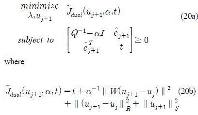
 j+1∈R(Q-1 – αI). Using the Schur complement and slack variable t∈R the optimized input can be found from equivalent semi-definite program (SDP) [20]
+ ∥ (uj+1 – uj∥2R + ∥ uj+1∥2R
3.2 Special case: Q = qI
In this subsection, the proposed robust ILC design is considered when Q = qI. The selection of weighting matrices as scaled identity matrices is common in practice, because it simplifies the tuning of the norm-optimal ILC algorithm and automatically guarantees monotonic convergence for the nominal case. An additional advantage of this choice is that it simplifies our robust problem leading to the analytical solution for the optimal parameter λ. In fact, if Q = qI, (19) yields the following optimal λ*as
and λ* = +∞, W(uj+1 – uj) = 0. The solution satisfies the constraint in (19.)
Consequently, problem (19) is reformulated as
where Jwc(uj+1) is the cost function with respect to the worst-case model uncertainty Δ*,
This problem can be solved effectively using convex programming [20].
3.3 Convergence
We now analyze convergence of the proposed robust ILC design with the case Q = qI. Define u*j+1 and e*j+1 as the optimal input and the corresponding tracking error of the robust ILC problem (22), respectively. Thu Jwc(u*j+1) ≤ Jwc(uj) , yielding
Moreover, for Δ ∈ Ψ0Δ we have
where e*j+1 = yd – P*Δuj+1 .As a result, we obtain the following inequality:
which shows the monotonic convergence of the robust ILC design. In addition, the relationship
demonstrates the monotonic convergence of the worst-case cost function.
4. Interpretation of the Results as Adaptive ILC
This section discusses the relationship between the developed robust approach and the classical norm-optimal ILC formulation. At first, the optimization problem (19) is rewritten as follows.
For the calculation of the optimal solution of this minimizing problem, the optimal input is achieved by differentiating the cost function with respect to, uj+1 yielding
where,
where
 j+1 are Lj+1 (λ + 1) dependent on λ + 1 and are calculated by using
After that, the optimal λ*j+1 is found from the following optimization problem:
This is a nonlinear optimization problem, and once λ*j+1 is calculated, the learning gains in the ILC law (28) are obtained yielding u*j+1. The parameters Qj+1 and Rj+1 in (29) can be updated by using λj+1 and u*j+1.
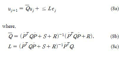
By comparing of the robust worst-case ILC controller described by (28)-(30) with classical ILC (8), the formula is the same except the weight matrices are updated trial-by-trial. Particularly, the adaptive controller depends on Qj+1 and Rj+1 while S remains trial-invariant. Moreover, if Q = qI then from (21) and (29) yields
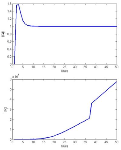
Hence, when the amount of uncertainty is very small, i.e.∥W∥≈ 0, the updated weights are approximately equal to the given Q and R. In addition, as an effect of the convergence of the robust ILC, i.e. uj+1 → uj as j→∞, the solution of λ in (18) shows that λj+1→ +∞. Thus ∥ Qj+1 ∥ converges to ∥Q∥, while ∥Rj+1∥ increases eventually to a very large value in the trial domain.
5. Simulation
Consider the uncertain plant: PΔ(s) =
 (s) + Δ(s) W(s) where the nominal model:
and the additive weighting transfer function is given by
For this simulation, an arbitrary stable unstructured uncertainty Δ(s) is selected as
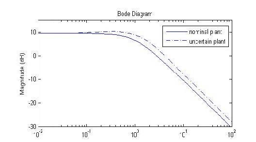
Figure 1 shows the Bode plots of the nominal model and the selected uncertain plant PΔ(s) with the given Δ(s) . Next, the nominal model, weight transfer function and un-structured uncertainty model are discretized with sampling time T = 0.002s, then lifted with N = 500 samples. Here, ∥Δ(q)∥∞ =1, while the lifted uncertainty model has its 2-norm: ∥Δ∥ ≈ 1.
Simulations of the proposed robust ILC algorithm are performed along 50 trials, and each trial starts from the same initial states.
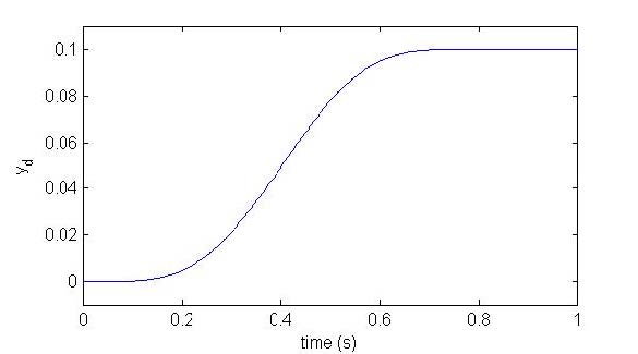
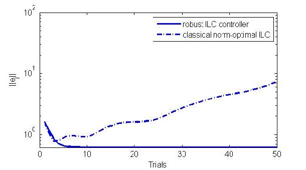
The reference trajectory is a smoothed step function, which is shown in Fig. 2. The weight matrices Q, R, and S are simply selected as scaled identity matrices I500, 0.8 ×I500, 0.0001 ×I500, respectively. Where In means I(n × n) matrix. The tracking errors obtained with the robust controller are shown in Fig. 3 (solid line). For comparison purposes, we also apply the same set of weight matrices Q; R; S to the classical norm-optimal ILC approach, and plot the results in Fig. 3 (dashed line). From the simulation results in Fig. 3, it can be seen that the robust ILC algorithm guarantees monotonic convergence of the tracking error. In contrast, the classical norm-optimal ILC design shows divergence of the tracking error. This demonstrates an advantage of the robust design over the classical norm-optimal ILC, where the robust ILC always achieves monotonic convergence.
In the next simulations, the equivalence between the proposed robust design and norm-optimal ILC with trial- varying weights is analyzed. Applying the equivalent adaptive ILC algorithm, the varying of Qj and Rj in the trial-domain were illustrated in Fig. 4. This figure confirms that ∥ Qj∥ decreases as j increases and eventually converges to ∥Q∥ as discussed in Section IV. On the other hand, ∥Rj∥ increases over the trials.
The changes in Qj and Rj result in a slower convergence. Hence, as the controller starts learning from previous trials, the convergence speed is decreased to obtain a robust algorithm.
6. Conclusion
The major contribution of this paper is a robust ILC design that can guarantee monotonic convergence in the presence of additive model uncertainty. The proposed robust ILC design approach corresponds to a convex optimization problem that can be solved efficiently. An interpretation of the robust ILC approach as an adaptive norm-optimal ILC with trial- varying learning gains is also investigated. The effectiveness of the proposed control scheme is confirmed from simulation results. The connection between robust ILC and adaptive norm-optimal ILC for both robustness and fast learning purposes will be further studied in the future works.
Acknowledgments
This paper is extended and updated from the short version that appeared in the Proceedings of the International symposium on Marine Engineering and Technology (ISMT 2013), held at BEXCO, Busan, orea on October 23-25, 2013.
References
-
D. A. Bristow, M. Tharayil, and A. G. Alleyne, “A survey of iterative learning control: a learning based method for high-performance tracking control”, IEEE Control Systems Magazine, 26, p96-114, June), (2006.
[https://doi.org/10.1109/MCS.2006.1636313]

-
H.-S. Ahn, Y. Chen, and K. Moore, “Iterative learning control: Brief survey and categorization”, Part C: Applications and Reviews, IEEE Transactions on Systems, Man, and Cybernetics, nov), 37, p1099-1121, (2007.
[https://doi.org/10.1109/TSMCC.2007.905759]

-
T. J. Harte, J. Hatonen, and D. H. Owens, “Discrete-time inverse model-based iterative learning control: stability, monotonicity and robustness”, International Journal of Control, 78(8), p577-586, (2005).
[https://doi.org/10.1080/00207170500111606]

-
R. W. Longman, “Iterative learning control and repetitive control for engineering practice”, International Journal of Control, 73, p930-954, (2000).
[https://doi.org/10.1080/002071700405905]

-
T. Donkers, J. van de Wijdeven, and O. Bosgra, “Robustness against model uncertainties of norm optimal iterative learning control”, Proceedings of the American Control Conference, (2008).
[https://doi.org/10.1109/ACC.2008.4587214]

-
E. Rogers, J. Lam, K. Galkowski, S. Xu, J. Wood, and D. Owens, “LMI based stability analysis and controller design for a class of 2D discrete linear systems”, Proceedings of the 40th IEEE Conference on Decision and Control, 5, p4457-4462, (2001).
[https://doi.org/10.1109/CDC.2001.980904]

-
D. Owens, and S. Daley, “Robust gradient iterative learning control: time and frequency domain conditions”, International Journal of Modeling, Identification and Control, 4(4), p315-322, (2008).
[https://doi.org/10.1504/IJMIC.2008.021471]

- K. Moore, Y. Chen, and H.-S. Ahn, “Algebraic H1 design of higher-order iterative learning controllers”, Proceedings of the IEEE International Symposium on Intelligent Control, june), p1207-1212, (2005.
-
D. Bristow, and A. Alleyne, “Monotonic convergence of iterative learning control for uncertain systems using a time-varying filter”, Automatic Control, IEEE Transactions on, 53, p582-585, march), (2008.
[https://doi.org/10.1109/TAC.2007.914252]

-
H.-S. Ahn, K. Moore, and Y. Chen, “Monotonic convergent iterative learning controller design based on interval model conversion”, IEEE Transactions on Automatic Control, Feb), 51, p366-371, (2006.
[https://doi.org/10.1109/TAC.2005.863498]

-
D. H. Nguyen, and D. Banjerdpongchai, “A convex optimization approach to robust iterative learning control for linear systems with time-varying parametric uncertainties”, Automatica, 47(9), p2039-2043, (2011).
[https://doi.org/10.1002/asjc.266]

-
N. Amann, D. H. Owens, E. Rogers, and A. Wahl, “An H1 approach to linear iterative learning control design”, International Journal of Adaptive Control and Signal processing, 10(6), p767-781, (1996).
[https://doi.org/10.1002/(SICI)1099-1115(199611)10:6<767::AID-ACS420>3.3.CO;2-C]

- D. Roover, “Synthesis of a robust iterative learning controller using an approach”, Proceedings of the 35th IEEE Conference on Decision and Control, 3, p3044-3049, dec), (1996.
-
K. L. Moore, H.-S. Ahn, and Y. Q. Chen, “Iteration domain optimal iterative learning controller design”, International Journal of Robust and Nonlinear Control, 18(10), p1001-1017, (2008).
[https://doi.org/10.1002/rnc.1231]

-
J. J. M. van de Wijdeven, M. C. F. Donkers, and O. H. Bosgra, “Iterative learning control for uncertain systems: Non-causal finite time interval robust control design”, International Journal of Robust and Nonlinear Control, 21(14), p1645-1666, (2011).
[https://doi.org/10.1002/rnc.1657]

- S. Skogestad, and I. Postlethwaite, Multivariable feedback control: analysis and design, John Wiley, (2005).
-
S. Gunnarsson, and Norrl Mikael, ¨ of , “On the design of ILC algorithms using optimization”, Automatica, 37(12), p2011-2016, (2001).
[https://doi.org/10.1016/S0005-1098(01)00154-6]

-
K. Barton, A. Alleyne, “A norm optimal approach to time-varying ILC with application to a multi-axis robotic testbed”, IEEE Transactions on Control Systems Technology, 19, p166-180, Jan), (2011.
[https://doi.org/10.1109/TCST.2010.2040476]

-
T. K. Nam, Dang Khanh Le, “A study on the control scheme of vibration isolator with electrical motor”, Journal of the Korean Society of Marine Engineering, 36(1), p133-140, (2012).
[https://doi.org/10.5916/jkosme.2012.36.1.133]

-
M. Norrlof, and S. Gunnarsson, “Time and frequency domain conver-gence properties in iterative learning control”, International Journal of Control, 75(14), p1114-1126, (2002).
[https://doi.org/10.1080/00207170210159122]

- S. Boyd, and L. Vandenberghe, Convex Optimization, Cambridge University Press, (2004).


