Turbulent properties in a mixed statistically stationary flow

1. Introduction

Mixing flows are widely used for the applications in many industry, such as mud separations in offshore engineering, For their applicability, man studies were carried out, especially by the use of measurement techniques [1][2]. For measurements, the stereoscopic PIV (SPIV) [3] has been used most widely as a three-dimensional measurement tool, since it provides high definition density of velocity vectors than other technique. As researches in the mixing flows, Chung et al. [4] used 2-D PIV technique to measure a stirred vessel flow. In this study, time-averaged 3D properties were obtained by using 2D PIV results along many vertical and horizontal planes. Kendra et al. [5] got volumetric three-components of velocity vector in a mixing tank in which a Rushton blade was rotated using the V3V technique for the analysis of the mixing flows. The measurement volume was limited to a certain size due to their capabilities. The velocity vectors obtained by the scanned stereoscopic PIV [6] give highly precise measurement results. In this study, a pseudo scanning stereoscopic PIV measurement was carried out by using three cameras for the measurements of the mixing flow in which an agitator was rotated at the tank bottom clockwise and counter-clockwise.

2. Experimentations

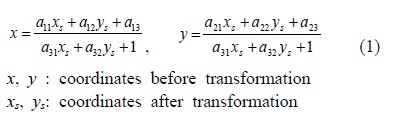
Figure 1 shows the experimental setup. At the bottom of the mixing tank (H= 60cm, D=60cm), an agitator which has 6 convex blades is rotating with variable speeds (maximum speed, 80 rpm) clockwise and counter-clockwise. As working fluids, water was filled up to 91mm from the top of the agitator. For stereoscopic PIV measurements, two cameras (1k x 1k, 500fps) were used. The third camera was used (1k x 1k, 500fps) for the measurement of rotational speed. The three cameras were synchronized each other for simultaneous measurements. A continuous laser (8W, 532nm) was used for visualization. Two-dimensional light sheet with a thickness of 5mm was generated via a cylindrical lens attached at the laser source. Nylon particles (d= 300μm, ρ =1.02) were used as tracers. The two cameras were calibrated before main experiments. To reduce the refraction effect of the circular water tank, a square outer tank box was installed and water was filled in the gap between the inner circular tank and the outer square tank. Further, to minimize the image aberration effect due to the misalignment between the camera lens plane and the tank wall, (2D) image transformation called warping transformation was made for the experimental images using the below Equation (1).

For camera calibration, 10 parameter method developed by Doh et. al [7] was used, in which 10 unknown parameters, 6 exterior parameters (l, α, β, γ, mx, my) and 4 interior parameters (c_x, c_y, k₁, k₂) were calculated. Detailed process for this calculation is well explained in the reference [7]. The calibration method in the present study is based on the pinhole model, and Equation (2) was used for constructing the relation between the land coordinate and the camera coordinate.

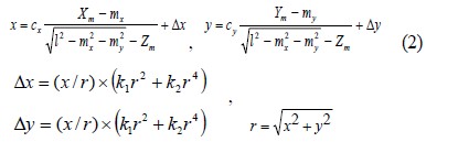
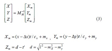
Here, c_x and c_y are the focal distances for the x and y components of the coordinate. Δx and Δy are the lens distortions. l refers to the distance between the origin O (0, 0, 0) and the principal point (X₀, Y₀, Z₀) of the camera. (x, y) represents the photographical coordinate of the image centroid of the calibration targets. (X_m, Y_m, Z_m) represent three dimensional coordinates of the object in the physical coordinate (land coordinate). m_x and m_y are misalignments between the coordinate centers of the two coordinates. After camera parameters had been calculated, the three dimensional coordinates (X, Y, Z) of the vector were calculated using the below Equation (3). The rotational transformation matrix, M_M, consists of the 10 camera parameters.

Here, t’ is the arbitrary coefficient and was obtained by the least square method. If the camera center is set to a vector (X₀, Y₀, Z₀), the collinear equation for one object (or particle) can be expressed as P(X, Y, Z ) = (a₁q + X₀, a₂q + Y₀, a₃q + Z₀), where q is an arbitrary vector. Here, a₁, a₂ and a₃ represent the corresponding term that can be reconstructed from Equation (3).

The cross-sectional points constructed from the following two collinear equations for the two cameras were defined as the 3-D positions in the absolute coordinate.

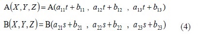
t and s were obtained by the least square method. Here, the coefficients (a₁₁, a₁₂, and a₁₃) and (b₁₁, b₁₂, and b₁₃) represent the corresponding terms that can be reconstructed from Equation (3) for the camera1, and (a₂₁, a₂₂, and a₂₃) and (b₂₁, b₂₂, and b₂₃) for the camera2. The final 3-D position of the object was calculated using the below Equation (5).

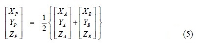
where (X_A, Y_A, Z_A) denotes the absolute coordinates for Camera ‘A’ defined by Equation (4),

Figure 1:

Measurement apparatus.

Figure 2:

Agitator, measured planes, and coordinates.

Figure 2 shows the shape of an agitator which mixes the water clockwise and counterclockwise with a sinusoidal mixing speed with maximum 80rpm. The measurement planes were set as shown in Figure 2(a), and the definition of the coordinates is shown in Figure 2(b). After the camera calibration, the tank was filled with water up to 91 mm height from the origin of the coordinate defined in Figure 2(b). The time consecutive images of the three cameras were captured by the three cameras and the two images of the camera 1 and the camera 2 were used for the calculation of 3D vector fields and the images of the camera 3 were used for the calculation of rotational speed. All cameras were synchronized. Three dimensional vector fields were obtained on the grids 60 x 20 at the visualized plane as defined in Figure 2(a). Figure 3 shows the rotational speed change of the agitator.

Figure 3:

Mixing speed change of the agitator.

Table 1:

Locations of the data sampling lines.

Table 2:

Coordinates of data sampling lines.

Figure 4:

Data sampling periods.

Figure 5:

3D phase averaged vector fields reconstructed at 10 locations.

Figure 6:

3D instantaneous vector fields measured at the vertical plane V1.

This data were calculated based on the PIV calculation using the images of the camera 3. Table 1 shows the physical locations of the data sampling planes. Table 2 is the physical coordinates where velocity vectors were sampled. Since the flow mixed by the agitator can be regarded as fully developed and symmetric flow for the rotation axis, i.e. statistically stationary flow, the velocity vectors can be reconstructed for the whole measurement volume just by taking phase averaging for the whole vector fields obtained at the same agitator’s locations. 200 instantaneous vector fields were averaged. Figure 4 shows the locations of the phase averaging.

3. Results and Discussion

Figure 7:

Distribution of TKE at four different mixing cycles at Figure 4(H1 plane).

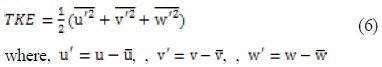
Figure 5(a) and Figure 5(b) show three dimensional reconstructed vector fields for the measurement plane H2 defined in Table 1 and Figure 2(a). These instantaneous vectors were reconstructed at 10 locations where one of the blades of the agitator as shown in Figure 2(a) passed between the blade’s angle of 60^o. 200 instantaneous measured vectors at the same location of the blade were averaged. This means that vectors show a phase averaged values. Figure 5(a) shows the phase averaged vector field at the instance of time ‘0’ as shown in Figure 4. Figure 5(a) shows the phase averaged vector field at the instance of time ‘4’ as shown in Figure 4. From these figures, it can be said that the mixed flows at the same rotational speeds have similar flow structures. Figure 6(a) and Figure 6(b) show the instantaneous vector fields measured at the vertical plane V1 defined in Table 1 and Figure 2(a) at the instances of time ‘0’ and time ‘4’. From these two instantaneous vector fields, it can be said that the flow structure at the same instance are similar each other, which enable that the flow structures are well organized and are strongly influenced by the agitator’s blade. Figure 7 shows the distribution of turbulent kinetic energy at the horizontal plane H1 defined in Table 1 and Figure 2(a). The turbulent kinetic energy (TKE) was calculated by using the below Equation (6).

Here, u, u’and denote the instantaneous value of measured vector, time averaged vector and fluctuation value, respectively. Since the figures were reconstructed on the condition that the flow inside of the mixing tank is statistically stationary and symmetric between the agitator’s 6 blades, the results show hexagonal symmetric structures. H2 plane is just over the location of the agitator’s blade. This means that the flow structures at H1 is strongly influenced by the agitator’s arrangement and shape. At every instance of mixing cycles, the flow structures are distinctively different each other. At the maximum mixing speed (80rpm) of the agitator, it can be seen that a ring-type high TKE distribution. This is due to the influence of the blade’s shape as shown in Figure 2(b). This means that the location of the top of the agitator is at the location of the ring. Figure 8 and Figure 9 show the distributions of the TKE at two different horizontal planes at (1/8)T and (3/8)T, respectively. From Figure 8(a) and Figure 8(b), it can be said that the flow at upper plane, which is close to the water surface, is strongly squeezed to counterclockwise near the tank wall at the time of (1/8)T. High TKE region is widely spread over the whole area except the tank center. This High TKE region moves to the center region along a circle. This fact implies that the mixed flow moves from the tank wall to the tank center while squeezed counterclockwise. This phenomenon can also be seen from the TKE distribution of the vertical plane V1 as shown in Figure 10. From Figure 10, it can also be said that the High TKE region moves from the tank wall toward the tank center, and this region is wrapped counterclockwise scrolling over the tank wall. This phenomenon can be found from Figure 6, too. Figure 11 shows the profiles of TKE along the lines defined as in Table 2. From Figure 11(a) and Figure 11(b), it can be said that the turbulent kinetic energy is higher at the area close to the tank wall compared to those at the center area. This fact is due to a strong counter rotating vortex flows produced by the agitator. From Figure 11(c) and Figure 11(d), it can also be evaluated that the TKE values are larger at outer region of the tank than those of the inner region. Further, the turbulent kinetic energy is uniform vertically along the wall. This implies that there is a strong vertical wall jet scrolling over the wall.

Figure 8:

Distribution of turbulent kinetic energy (TKE) at two measurement planes (H1, H2) at the instance of mixing cycle (1/8)T.

Figure 9:

Distribution of turbulent kinetic energy (TKE) at two measurement planes (H1, H2) at the instance of mixing cycle (3/8)T.

Figure 10:

Distribution of turbulent kinetic energy (TKE) at the vertical plane (V1) at two instances of mixing cycles.

Figure 11:

Profiles of turbulent kinetic energy at four different sampling lines in Table 2 at the instance of mixing cycle (1/8)T.

4. Summary

The turbulent properties in the mixing flow in the statistically stationary mixing flow were measured by a pseudo volumetric stereoscopic PIV (SPIV) system. Large difference of the mixing flow was seen between (1/8)T and (3/8)T. The profiles of the turbulent kinetic energy (TKE) were similar each other when the rotation speeds were the same RPM even if acceleration and deceleration occurred. It was verified that the distribution patterns of the TKE inside of the mixing flow were strongly influenced by the agitator’s location and shape. It was shown that there was a scrolling jet having large TKE values along the tank wall, and it was wrapped toward the tank centre from the tank wall.

Acknowledgments

This work was supported by the National Research Foundation Grant funded by the Korean Government (MEST) (No. 2008-0060153) and this work is the outcome of a Manpower Development Program for Marine Energy by the Ministry of Oceans and Fisheries.

References

• D. H. Doh, D. H. Kim, K. R. Cho, Y. B. Cho, T. Saga, and T. Kobayashi, “Development of genetic algorithm based 3D-PTV technique”, Journal of Visualization, 5(3), p243-254, (2002). [https://doi.org/10.1007/BF03182332]
• F. Pereira, H. Stuer, EC. Graff, and M. Gharib, “Two-frame 3D particle tracking”, Measurement Science and Technology, (2006), 17(7), p1680-1692. [https://doi.org/10.1088/0957-0233/17/7/006]
• S. M. Soloff, R. J. Adrian, and Z. C. Liu, “Distortion compensation for generalized stereoscopic particle image velocimetry”, Measurement Science and Technology, 8(12), p1441-1454, (1997). [https://doi.org/10.1088/0957-0233/8/12/008]
• K. H. Chung, M. Barigou, and M. J. H. Simmons, “Reconstruction of 3-D flow field inside miniature stirred vessels using a 2-D PIV technique”, Chemical Engineering Research & Design, 85(5), p560-567, (2007). [https://doi.org/10.1205/cherd06165]
• V. S. Kendra, H. David, T. Daniel, and W. Geoffrey, “Volumetric three-component velocimetry measurements of the turbulent flow around a rushton turbine”, Experiments in Fluids, 48(1), p167-183, (2010). [https://doi.org/10.1007/s00348-009-0711-9]
• T. Hori, and J. Sakakibara, “High-speed scanning stereoscopic PIV for 3D vorticity measurement in liquids”, Measurement Science and Technology, 15(6), p1067-1078, (2004). [https://doi.org/10.1088/0957-0233/15/6/005]
• D. H. Doh, T. G. Hwang, and T. Saga, “3D-PTV measurements of the wake of a sphere”, Measurement Science and Technology, 15(6), p1059-1066, (2004). [https://doi.org/10.1088/0957-0233/15/6/004]