Anomaly detection of unbalanced rotating shaft based on deep learning and thresholds
Copyright © The Korean Society of Marine Engineering
This is an Open Access article distributed under the terms of the Creative Commons Attribution Non-Commercial License (http://creativecommons.org/licenses/by-nc/3.0), which permits unrestricted non-commercial use, distribution, and reproduction in any medium, provided the original work is properly cited.
Abstract
Motors are important machines used in various industries. They provide power to various pumps, air compressors, refrigeration plants, purifiers, and air-conditioning plants. However, the motor may not be optimally coupled with the driven machinery during the repair process, and the bearings may become damaged over time as the machine operates. These problems can cause an imbalance in the motor shaft, thus resulting in vibrations. Therefore, vibrations and abnormal indicators must be detected timely to ensure machine safety. A deep-learning model for anomaly detection based on publicly available bearing data was developed in this study. Bearing data from various experiments were plotted and their characteristics were analyzed. Additionally, the vibration amplitude graphs of certain sections were saved as images. The saved images were categorized into normal and abnormal, and then classified using a convolutional neural network (CNN) model. Evaluation of the model performance on the test set for the trained CNN model shows an accuracy of 0.95, which indicates that the model performs well in distinguishing between normal and abnormal vibration amplitudes. Furthermore, anomaly detection based on vibration-amplitude threshold values was performed.
Keywords:
Bearing, Anomaly detection, Deep learning, Convolutional neural network, Threshold1. Introduction
Most components on ships, except for the main diesel engine, diesel generator, and boiler, obtain power from motors. These motors are typically connected to pumps, air compressors, provision refrigeration plants, purifiers, and air-conditioning plants via coupling or pulleys and V-belts on ships. The abovementioned components must be disconnected from the motor for their periodic maintenance.
However, the connection between the machine and motor may be unbalanced depending on the skill level of the marine engineer. For example, the heights of the shafts on the motor and pump sides may not match, or, the left and right balances of the shafts on the motor and pump sides may not match. In some cases, these problems can occur simultaneously.
In existing ships, the ampere gauge or sound is used to determine if the connection between the machine and motor is not optimal by confirming a high ampere or abnormal noise. However, if anomaly detection is not performed in advance, then damage can accumulate at the motor bearing, pump, or machine. Therefore, an intelligent model that detects abnormalities based on artificial intelligence and big data received from sensors must be developed.
Jin et al. detected bearing anomalies and predicted its remaining useful life using an autoregressive model, a health index, a threshold based on the Box–Cox transformation, a nonlinear model, and a Kalman filter[1]. König et al. classified the multivariant wear behavior of sliding bearings based on acoustic emissions. Machine-learning methods were used to detect anomalies and convolutional neural networks (CNNs) were used for multiclass classification[2]. Hiruta et al. created a power spectrum from current sensor signals and employed a Gaussian mixture model to learn the normal conditions of a motor bearing. Hiruta et al. detected a motor-bearing failure mode caused by insufficient grease by adopting unsupervised learning[3]. Zhang et al. proposed a semi-supervised learning approach for bearing anomaly detection using a variational autoencoder based on the Case Western Reserve University bearing dataset and the University of Cincinnati’s Center for Intelligent Maintenance Systems dataset[4]. Lee et al. used a stacked CNN to extract spatial fea-tures from vibration sensor data, a stacked gated recurrent unit to learn temporal features, and a regression layer to predict anomaly de-tection based on bearing data from the National Aeronautics and Space Administration (NASA) prognostics data repository[5]. Geor-goulas et al. performed empirical mode decomposition and the Hilbert Huang transform to extract a compact feature set[6]. Subsequent-ly, they used a hybrid ensemble detector trained with normal bearing data to detect deviations from the normal condition. Ahmad et al. used an autoencoder model to learn the characteristics of normal vibration signals and a threshold to perform anomaly detection based on error values[7]. Roy et al. used an autoencoder and an online sequential extreme-learning machine network to detect the bearing health states of the NASA bearing dataset[8].
In several previous studies, publicly available data were used for bearing anomaly detection. Using public data eliminates the necessi-ty to purchase expensive equipment and sensors for experiments, reduces time in conducting experiments, and yields verified, high-quality data. Therefore, public data were used to analyze and develop algorithms for bearing anomaly detection. The remainder of this paper is organized as follows: Section 2 describes the process of obtaining data from the experiment. Section 3 presents an analysis of the data obtained. Section 4 describes the preprocessing. Chapter 5 explains the process of constructing a CNN and threshold-based algorithms. Section 6 presents the prediction results of two anomaly-detection algorithms. Finally, Section 7 summarizes the important findings of this study.
2. Data Acquisition
2.1 Acquisition of Data
Data labeled under “Vibration analysis on rotating shaft” were obtained from the “Kaggle” website, which provides free access to high-quality data worldwide[9]. The data were obtained from an original study and republished in “Kaggle”[10].
2.2 Experimental Setup
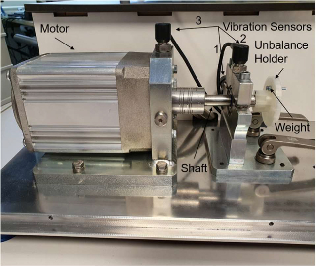
Mey et al. established an experiment setup, as shown in Figure 1, to perform data acquisition.
As shown in Figure 1, all the main components used in the experiment were fixed to an aluminum base plate. The motor shaft was connected to another shaft through coupling, and an unbalanced holder was installed at the end of the shaft to provide an unbalanced condition. The unbalanced holder featured a hole, into which weights can be inserted to create an unbalanced condition. The shaft was supported by a roller bearing and roller-bearing block. Vibration 1 and 2 sensors were installed on the side and top of the roller bearing block, respectively. Vibration 3 sensor was installed at the top of the motor block. Signals from the vibration sensors were obtained using a four-channel data acquisition system. The rotational speed of the motor was measured using a frequency counter in the data-acquisition system. The details of the main components used in the experiments are listed in Table 1.
2.3 Data-Acquisition Process
The details of the weights installed on the unbalanced holder to unbalance the shaft are presented in Table 2. Herein, “D” and “E” re-fer to experiments for development and evaluation, respectively. Although five different weights were used, 10 experiments were conducted. "0D/0E" indicates a normal state in which weights are not installed. From "1D/1E" to "3D/3E", the mass weight was the same, whereas the mass radius differed. "3D/3E" and "4D/4E" were tested under the same mass radius but different mass weights.
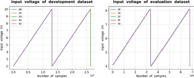
The rotational speed varies depending on the voltage applied to the motor controller. Therefore, in the development experiment, the voltage was increased from 2.0 to 10.05 V; each step lasted 20 s, and the difference between the steps was 0.05 V. In the evaluation experiment, the voltage was increased from 4.0 to 8.1 V; each step lasted 20 s, and the difference between the steps was 0.1 V.
3. Data Analysis
3.1 Analysis of Input Voltage
Figure 2 shows the input voltages for the development and evaluation datasets. The voltage was increased for each dataset to the val-ues mentioned above, and the same experiment was conducted twice. For the evaluation dataset, the difference between the steps was twice that for the development dataset; therefore, the graph shape showed steps.
3.2 Analysis of Vibration-Sensor Amplitude
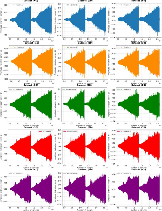
Figure 3 shows the three vibration amplitudes of five experiments for the development dataset. A comparison of the vibration ampli-tudes from the three different sensors for the five experiments showed that they exhibited different patterns.
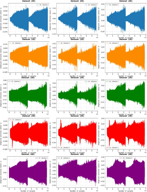
Figure 4 shows the three vibration amplitudes of the five experiments for the evaluation dataset. A comparison between the graphs of the evaluation and development datasets show a larger vibration amplitude for the evaluation dataset. Similar to the case of the develop-ment dataset, different patterns were observed in the evaluation dataset when comparing the amplitude between the three vibration sen-sors and the amplitude between the five experiments.
At the beginning of the experiment for the development and evaluation datasets, we observed significant differences between the 0D and 4D datasets; however, this aspect was not considered because it was not observed in the stable amplitude state.
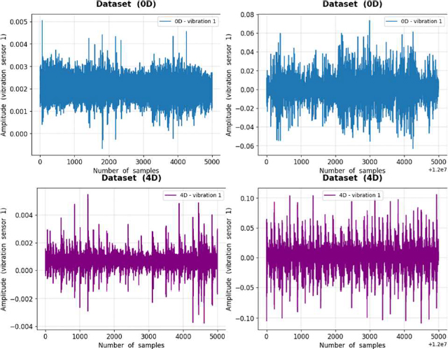
Because the sampling rate of the data-acquisition system was 4,096 values per second, the data at the starting (0th to 5,000th samples) and end (12,000,000th to 12,005,000th samples) points were plotted, as shown in Figure 5 to verify the data pattern per second. No specific pattern was observed within 1 s and the graphs showed a discontinuous vibration amplitude. At the starting point, the amplitude was uniform; however, at the end point, the amplitude fluctuated significantly. This pattern was similarly observed in Figure 3 and Figure 4.
4. Data Preprocessing
In this study, the 0D dataset of vibration sensor 1, which was in the normal condition, and the 4D dataset of vibration sensor 1, which was in the most unbalanced condition, were used for anomaly detection. The evaluation dataset was excluded because the input voltage was within the development dataset. However, the anomaly detection of the evaluation dataset can be solved using the same method as that used in this study.
As shown in Figure 3, a difference was clearly indicated between 0D and 4D beginning from the 8,000,000th sample. At the begin-ning of the experiment, a significant difference was observed between 0D and 4D; however, this was not considered because it did not appear in a stable amplitude state. Accordingly, data from the 8,000,000th to 12,000,000th samples were used, which indicated the end point of the first experiment.
Using the sliding-window method, 100 images were saved each for 0D and 4D with an interval of 40,000 samples. Because 4,096 samples per second were saved by the data-acquisition system, one image represented an amplitude of approximately 10 s. The image was saved at a pixel size of 256 × 256. For the 0D and 4D datasets, 70% was allocated as the training set and 30% into the test set to train the CNN model.
In Figure 6, (a and b) represent the 1st and 100th images for the 0D dataset, respectively, and (c and d) represent the 1st and 100th images for the 4D dataset, respectively. The 100th image shows a different pattern compared with the 1st image, as the rpm of the 100th image is greater than that of the 1st image.
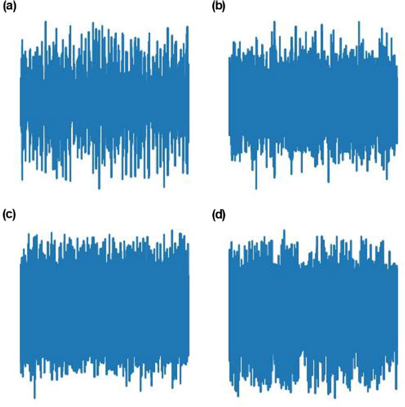
1st (left) and 100th (right) images of vibration amplitude for 0D (top) and 4D (bottom) datasets of vibration sensor 1
During CNN model training, the axes, lines, and letters can provide unnecessary information to the model; therefore, only the vibra-tion amplitude was saved as an image, as shown in Figure 6.
5. Modeling
5.1 CNN-Based Anomaly Detection
The CNN is a deep-learning technology that is primarily used to extract features from images. It gradually extracts features via convo-lutional computing using several filters. A CNN comprises an input layer, convolution and pooling operations, full connections, and an output layer; dropout layers are occasionally added to increase the generalization performance and prevent overfitting[11][12].
The 0D images were normal, whereas the 4D images were abnormal; the normal and abnormal images were labeled 0 and 1, respec-tively. As input to the CNN model, training images of size (256, 256, 3) were stacked. Consequently, 70% of the normal and abnormal images were accumulated to create an array of different size (140, 256, 256, 3). Accordingly, a label array of size (140, 1) comprising 0s and 1s was created. An array of size (60, 256, 256, 3) comprising 30% normal and abnormal images was created for testing, and an array of size (60, 1) was created as a test label. Normalization was performed by dividing the values of the training and test set arrays by 255.
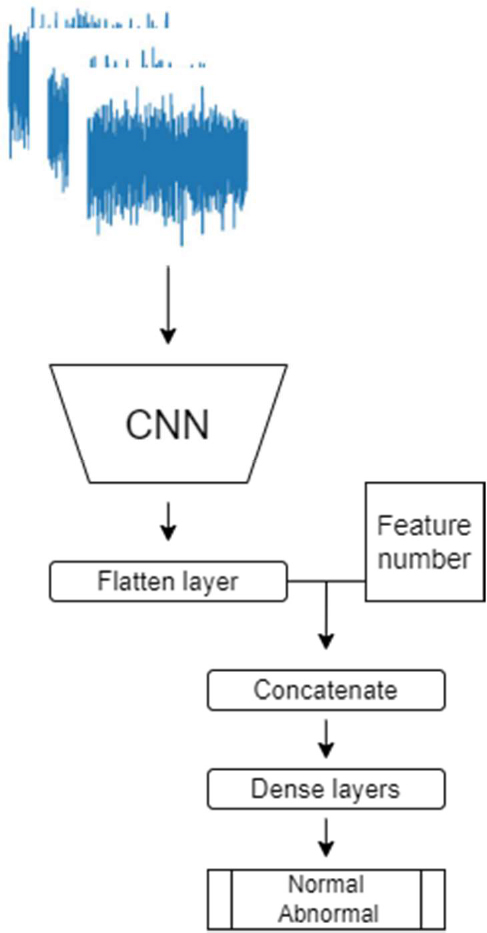
As images from various rpm ranges were used in this study, the CNN model must reflect the rpm range to which the image belongs. Therefore, a feature number was used, as shown in Figure 7. The 100 images were divided into 10 sections, and numbers 1–10 were used as feature numbers in the order from low to high rpm.
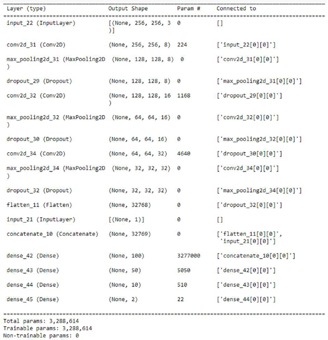
The process for modeling the CNN is as follows: The CNN model comprised four Conv2D, MaxPooling2D, and Dropout layers, and the outputs of these layers are passed through a flattened layer. The filters of the Conv2D layers were used sequentially: 8, 16, 32, and 32. The kernel size was 3 × 3, the activation function was a rectified linear unit (ReLU), and the padding was the same. The pooling size of MaxPooling2D was set to 2 × 2, and the dropout rate was set to 25%. The vectors of the flattened layer and feature number were concatenated. The concatenated vectors were input into dense layers containing 100, 50, 10, and 2 neurons. In the last dense layer, the sigmoid function was used as an activation function to output normal and abnormal conditions, and the ReLU was used in the remaining three dense layers. “Sparse_categorical_crossentropy” was used as the loss function, Adam was used as the optimizer, and accuracy was used as the training-performance metric. The CNN model was constructed using the TensorFlow and Keras libraries, and its detailed architecture is shown in Figure 8.
The CNN model was trained with image and feature number arrays as the input and label arrays as the output, with a batch size of 30 for 100 epochs.
5.2 Threshold-Based Anomaly Detection
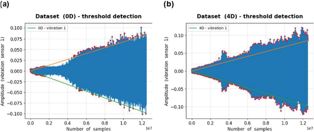
As shown in Figure 3, the first cycle ended at approximately the 12,500,000th sample. Therefore, the maximum and minimum values from the 12,450,000th to the 12,550,000th sample among the data from the 0D experiment for vibration sensor 1 were obtained. The maximum and minimum value were 0.084621906 and -0.098769665 for the 12,453,255th and 12,514,162th samples, respectively. The line passing through these points, based on the origin, was used as the threshold.
6. Result and Discussion
6.1 CNN-Based Anomaly Detection
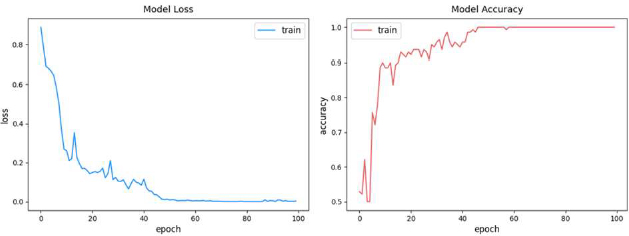
Figure 9 shows the training loss and accuracy for 100 epochs of the CNN model. The loss decreased gradually and remained low af-ter approximately 50 epochs. Contrary to the model-loss graph, the accuracy was approximately one-half that of the probability predic-tion at the beginning; however, the accuracy was 1 after 50 epochs.
To evaluate the performance of the trained CNN model, we input test image and feature number arrays into the trained CNN model, and the prediction results for the testing set were compared using the test labels. The accuracy value was 0.95, thereby indicating that the trained CNN model performed well in distinguishing between normal and unbalanced conditions for the rotating shaft.
6.2 Threshold-Based Anomaly Detection
For the 0D dataset, 75,824 data points exceed the threshold line, as shown in Figure 10 (a). The orange and green lines represent the threshold lines based on the maximum and minimum values, respectively. The red dots represent data points that exceed the threshold lines.
For the 4D dataset, 108,475 data points exceeded the threshold lines, which was 32,651 more data points than that exceeded by the 0D dataset. Therefore, we confirmed that anomaly detection can be performed, based on the fact that more data points exceeded the threshold lines as compared with the normal condition.
7. Conclusion
Motors are important machines that convert electrical energy into mechanical power and are used in various industrial fields. Many motors are installed on ships, where power is obtained using electrical energy generated by diesel generators. Motors are used to drive various pumps, air compressors, provision refrigeration plants, purifiers, and air-conditioning plants.
Motor vibration can arise due to the deterioration of bearing performance over time or from a suboptimal connection between the mo-tor and driven machinery. Detecting these issues in advance is crucial for extending the lifespans of motors, bearings, and machinery.
Hence, we used publicly available high-quality bearing data for this study. Bearing data were plotted, and their characteristics were analyzed. Data from normal and extremely unbalanced conditions were used in conjunction with a CNN model to detect normal and abnormal conditions. The vibration-amplitude graphs were saved as images for each rpm section of the bearing data.
Additionally, we concatenated the feature-number vector with the flattened-layer vector of a convolutional network such that the CNN model can predict the results and thus reflect image classification based on various rpm sections.
The training process of the CNN model was confirmed, and the prediction performance of the testing set showed an accuracy of 0.95, which indicated its effectiveness in detecting normal and abnormal vibration amplitudes.
Anomaly detection was performed based on the vibration-amplitude threshold values under normal conditions. The result showed that the 4D dataset had 32,651 more data points that exceeded the threshold lines compared with the 0D dataset.
Therefore, based on the methodology used in this study, anomaly detection can be performed based on 1) vibration amplitude images of the motor bearing, whose rpm can vary, and the feature number based on the rpm section; and 2) threshold values.
Acknowledgments
This research was supported by the Autonomous Ship Technology Development Program [20016140] funded by the Ministry of Trade, Industry, & Energy (MOTIE, Korea); and the National Research Foundation of Korea (NRF) grant funded by the Korea government (MSIT) [NRF-2022R1F1A1073764]; and the ‘Technology development Program [S3366238]’ funded by the Ministry of SMEs and Startups (MSS, Korea).
Author Contributions
Conceptualization, M. H. Park and W. J. Lee; Methodology, M. H. Park; Formal Analysis, M. H. Park; Investigation, M. H. Park; Writing-Original Draft Preparation, M. H. Park; Writing-Review & Editing, M. H. Park and W. J. Lee; Visualization, M. H. Park; Supervision, W. J. Lee; Project Administration, W. J. Lee; Funding Acquisition, W. J. Lee.
References
-
X. Jin, Y. Sun, Z. Que, Y. Wang, and T. W. S. Chow, “Anomaly detection and fault prognosis for bearings,” IEEE Transactions on Instrumentation and Measurement, vol. 65, no. 9, pp. 2046-2054, 2016.
[https://doi.org/10.1109/TIM.2016.2570398]

-
F. König, C. Sous, A. Ouald Chaib, and G. Jacobs, “Machine learning based anomaly detection and classification of acoustic emission events for wear monitoring in sliding bearing systems,” Tribology International, vol. 155, 2021.
[https://doi.org/10.1016/j.triboint.2020.106811]

-
T. Hiruta, K. Maki, T. Kato, and Y. Umeda, “Unsupervised learning based diagnosis model for anomaly detection of motor bearing with current data,” Procedia CIRP, vol. 98, pp. 336-341, 2021.
[https://doi.org/10.1016/j.procir.2021.01.113]

- S. Zhang, F. Ye, B. Wang, and T. G. Habetler, “Semi-supervised learning of bearing anomaly detection via deep variational autoencoders, arXiv preprint arXiv:1912.01096, , 2019.
-
K. Lee, J. K. Kim, J. Kim, K. Hur, and H. Kim, “CNN and GRU combination scheme for bearing anomaly detection in rotating machinery health monitoring,” 1st IEEE International Conference on Knowledge Innovation and Invention, ICKII 2018, pp. 102-105, 2018.
[https://doi.org/10.1109/ICKII.2018.8569155]

-
G. Georgoulas, T. Loutas, C. D. Stylios, and V. Kostopoulos, “Bearing fault detection based on hybrid ensemble detector and empirical mode decomposition,” Mechanical Systems and Signal Processing, vol. 41, no. 1-2, pp. 510-525, 2013.
[https://doi.org/10.1016/j.ymssp.2013.02.020]

-
S. Ahmad, K. Styp-Rekowski, S. Nedelkoski, and O. Kao, “Autoencoder-based condition monitoring and anomaly detection method for rotating machines,” 2020 IEEE International Conference on Big Data, pp. 4093-4102, 2020.
[https://doi.org/10.1109/BigData50022.2020.9378015]

-
M. Roy, S. K. Bose, B. Kar, P. K. Gopalakrishnan, and A. Basu, “A stacked autoencoder neural network based automated feature extraction method for anomaly detection in on-line condition monitoring,” 2018 IEEE Symposium Series on Computational Intelligence (SSCI), pp. 1501-1507, 2018.
[https://doi.org/10.1109/SSCI.2018.8628810]

- JISHNU, Vibration Analysis on Rotating Shaft, https://www.kaggle.com/datasets/jishnukoliyadan/vibration-analysis-on-rotating-shaft/data, , published 2022.
-
O. Mey, W. Neudeck, A. Schneider, and O. Enge-Rosenblatt, “Machine learning-based unbalance detection of a rotating shaft using vibration data,” IEEE International Conference on Emerging Technologies and Factory Automation, pp. 1610-1617, 2020.
[https://doi.org/10.1109/ETFA46521.2020.9212000]

-
M. H. Park, J. S. Park, and W. J. Lee, “Toward optimized operation of freshwater generator using computer vision, and its economic and environmental benefits,” Desalination. vol. 573, 2024.
[https://doi.org/10.1016/j.desal.2023.117214]

-
M. H. Park MH, S. Chakraborty, Q. D. Vuong, et al., “Anomaly detection based on time series data of hydraulic accumulator,” Sensors, vol. 22, no. 23, 2022.
[https://doi.org/10.3390/s22239428]


