Improving colorization through denoiser with MLP
Copyright ⓒ The Korean Society of Marine Engineering
This is an Open Access article distributed under the terms of the Creative Commons Attribution Non-Commercial License (http://creativecommons.org/licenses/by-nc/3.0), which permits unrestricted non-commercial use, distribution, and reproduction in any medium, provided the original work is properly cited.
Abstract
Colorizing black and white photos and movies enhances the old versions, and make them more interesting to see. Therefore, we became interested in image colorization, which plays an essential role in the field of computer vision. Recently, deep learning techniques for image colorization have progressed remarkably. In this study, colorization is carried out using a novel deep learning model for vivid coloring. The model consists of two components: Pix2Pix as a generative adversarial network (GAN), and the multilayer perceptron (MLP) of a denoiser. The Pix2Pix primarily generates the color image for a given grayscale image as input, and the MLP transforms the colored image into a vivid color image by filtering out noise. In our experiments, the grayscale images used as input images were images of natural objects and artifacts. We observed that the predicted images provided as output images were more neatly colored through the proposed method.
Keywords:
Colorization, Color constancy, GAN, Pix2pix, Back propagation1. Introduction
The color of an object is determined by the wavelength of the reflected light, as affected by the physical properties of the object. To classify and express colors on a computer, we use RGB-like color models that mathematically describe colors. Colorization is the process of adding plausible color information to grayscale images [1][2]. Colorization has become common, and restoring grayscale images to color images can provide a more lively and special effect with the advent of digital image processing.
There are many benefits in colorizing images: 1) colorizing grayscale images and videos enhance the old versions, making them more interesting to see; and 2) colorizing night vision pictures makes them appear more vividly for autonomous driving and military applications. Image colorization can also be used to help a user to analyze an image. However, it is costly and time-consuming if image colorization must be performed manually by many artists. Recently, deep learning techniques [3][4] have progressed remarkably for image colorization.
The goal of a colorization model is to convert a grayscale image into a more natural color image by guessing colors through learning. In this paper, we propose a novel deep learning model for colorization. Basically, the model converts grayscale images into their color images using Pix2Pix model [5], which is a generative adversarial network (GAN) and an approach to training a deep convolutional neural network (CNN) for image-to-image translation tasks. Then, we use a denoiser with a multi-layer perceptron (MLP) to gradually improve the performance. An improved result can be extracted by minimizing the gap between the generated images and original images when viewing them. Moreover, our approach can successfully color high-level image components. In our experiments, the input grayscale images were images of natural objects and artifacts, and output images of predicted images were neatly colored through the proposed method. Also, an image quality measurement between the original color image and an image extracted by our method showed excellent results.
The rest of this paper is organized as follows. Section 2 presents the related works for colorization in brief. Section 3 describes the proposed method for colorization using Pix2pix and the MLP to improve the performance of colorization. In Section 4, we discuss the empirical results. Finally, Section 5 summarizes the work described herein and draws some conclusions and directions for future research.
2. Related Works for Colorization
In this section, we will briefly describe the vanilla GAN [6][7] of a well-known image generation model, a deep convolution GAN (DCGAN) of a GAN using a CNN, and a conditional GAN (CGAN) for feeding the data conditioned on certain factors, in order.
2.1 Vanilla generative adversarial network (GAN)
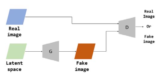
GAN [6][7] is one of the well-known generation models, and is a model that can generate data or samples with a pseudo-distribution Pmodel(x) generated by learning using learning data with a specific probability distribution Pdata(x). The GAN is an unsupervised learning model in which a Generator (G) and Discriminator (D) interact. G plays a role in generating data and deceiving D, and D plays a role in uncovering the falsehood of the image generated from G, as shown in Figure 1.
First, looking at D, it is distinguished whether the input given to the role of D is real data. Given the Data x as input, the output D(x) of D returns the probability that x is real data. The role of G is to create fake data that is so real that it is impossible to tell whether D is real. When the Latent space is given as shown in the figure above, a fake image G(z) is generated through G. If such G(z) is given again as input of D, D(G(z)) returns the probability that G(z) is real data.
| (1) |
From Equation (1) above, Discriminator D estimates that when actual data enters the output, the result is close to 1 and when fake data created by G enters, the result is close to 0. The GAN learns in this way from G and D alternately. G makes it possible for D to create fake data that is indistinguishable, and D makes it possible to find a balance point by learning G to distinguish between any fake data well.
2.2 Deep convolution GAN (DCGAN)
To solve the well-known poor stability of the GAN, the DCGAN [8], which applies a CNN, announced a model with an optimal structure. It was confirmed through experiments that applying the CNN to the original GAN alone cannot achieve sufficiently good results. Here are five methods applied in the vanilla GAN to produce optimal results: 1) remove the pooling layer and adjust the size of the feature-map using stridden convolution; 2) apply batch normalization; 3) remove the fully connected hidden layer; 4) Use the tanh function as the active function of the output terminal of the generator; and 5) use the rectified linear unit as the active function of the Discriminator.
2.3 Conditional GAN (CGAN)
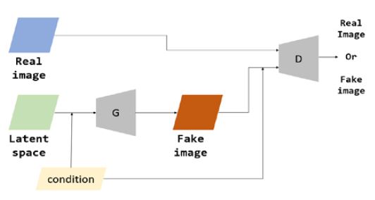
The CGAN [9]-[11] is a method of adding any condition y that can control the generation conditions to the original GAN, as shown in Figure 2. It can add information indicating a specific condition to the Generator and Discriminator. In fact, the effect of the condition occurs, and the type of output value is determined based on the value set during back-propagation when learning is performed. Later, the result can be manipulated by adding a condition value to the Generator. In the case of the Generator, the condition is accepted as an indicator of what to output, whereas the Discriminator accepts the condition and predicts what will come. It is used to adjust the pair between condition and real data, condition and fake data.
| (2) |
The value function as shown in Equation (2) of the CGAN is the same as Equation (1) of the vanilla GAN, except that only the input variables x and z enter as conditional variables x|y and z|y. In Equation (2), y can have various forms, as the form of y is not specifically defined. For example, if one wants to generate a desired number in MNIST, which recognizes cursive numbers, an additional label corresponding to the class of numbers can be added. In this study, the condition is the grayscale image.
3. Colorization through Denoiser with MLP
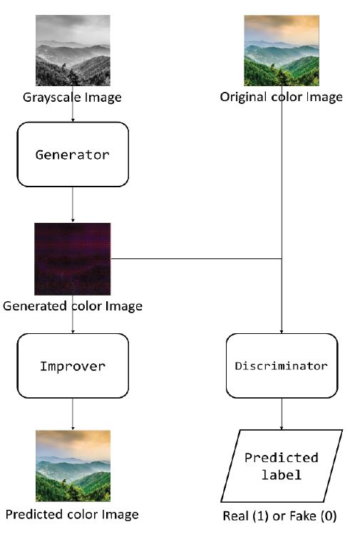
Figure 3 shows the overall architecture of the proposed model, which converts grayscale images into visually acceptable color images. The model consists of two components: the Pix2Pix model of the GAN and the MLP model of the denoiser. The Pix2Pix model [5] is a GAN and an approach to training a deep convolutional neural network for image-to-image translation tasks. The MLP transforms the colored image into a vivid color image by filtering out noise and then improving the performance. The models are described in detail in sequential subsections.
3.1 Generator
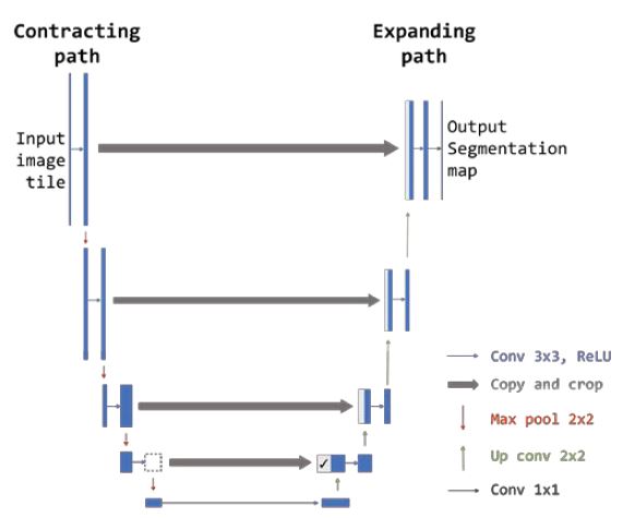
The Generator uses the structure of U-Net [12], as shown in Figure 4. The U-Net comprises an encoder-decoder with skip connections between mirrored layers in both the stacks. In this study, the input of U-Net is grayscale images and the output is colored images. The U-Net enables colorization even with a small number of data. Unlike an autoencoder of an encoder-decoder, this increases speed and solves the trade-off between context recognition and localization.
Context means the relationship between neighboring image pixels, and it can be seen as understanding the context of the overall image by looking at a part of the image. In addition, the trade-off is that it is easy to understand the context if a wide range of images is recognized at once, but then localization is not performed properly, so which pixel is which label is not recognized in detail. Conversely, if the range is narrowed, detailed localization is possible, but the context recognition rate is lowered. So, U-Net uses the following: 1) a patch search method rather than a sliding window; and 2) the context of the image is captured in the contracting path. In addition, after upsampling the feature-map in the expanding path, it is combined with the context of the feature-map captured in the contracting path to increase the accuracy of localization. Through these two processes, the speed is improved and trade-offs are resolved. From the left contracting path in Figure 4 above, convolution and pooling are performed to increase the number of channels in the feature-map by two times at each step, but while downsampling the size by two times. That is, it is small and sturdy. Next, the right expanding path goes through the contracting path, and the feature-map is downsampling so the resolution is much lower. Upsampling is performed several times to increase the resolution, i.e., to change the coarse-map into a dense-map.
U-Net uses the skip-connection concept, which combines the feature-map of the shallow layer with the feature-map of the deep layer. Here, the feature-map of the previous step before pooling is copied in the contracting path and concatenated to the corresponding feature-map in the expanding path. Note that missing data many occur if the size of the feature-map of the expanding path is smaller than the feature-map of the contracting path. So, for image correction, the middle part is cropped to an appropriate size, re-adjusted to a slightly smaller image, and attached. In the expanding path, after the upsampling step, the copy and crop and concatenate process is repeated at every step. Accordingly, convolution is performed in a state where the two feature-maps are superimposed. The features are fused to each other, resulting in better labeling of the values in the same pixel in this process.
3.2 Discriminator
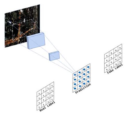
The Discriminator use the structure of PatchGAN as shown in Figure 5. Whereas the original Discriminator makes a fake/real judgment for the entire image, PatchGAN divides the image created by the Generator into small patches and determines the authenticity of the patches as fake/real. That is, a patch size of an appropriate size corresponding to the range in which the correlation relationship is maintained is determined, and the patches are mostly learned in the real direction. Here, the patch size can be viewed as a hyperparameter because it must include the overall image size and an appropriate range in which a correlation between a specific pixel and other pixels exists in the entire image.
Also, PatchGAN makes it possible to model an image as one Markov random field (MRF), because it assumes that pixels farther away than the patch diameter are independent of each other. MRF is an undirected graph model and is used to analyze images through Bayesian modeling. It has local, not temporal, Markov properties between random fields, so only the neighboring pixels are considered and the rest are not taken into account.
In other words, PatchGAN does not judge by looking at the entire data to identify one part of the data, but by identifying and judging the relationship with neighboring data.
By using this structure, more detailed high-level features can be well-captured in the image, and blur can be covered to some extent. Also, the number of parameters is much smaller because the operation is performed while the sliding window passes. This results in a faster computation speed and flexibility in terms of structure, as it is not affected by the overall image size.
3.3 Improver
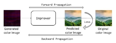
The Improver uses the structure of the MLP, as shown in Figure 6. The input and the output of the Improver are the color images generated by Generator and original color images, respectively. The Improver plays the central role of a de-noiser in the performance improvement. The MLP is trained by the back-propagation algorithm, which is a method of updating weights from back to forward to reduce errors present in the final output. In this study, the weights are updated by comparing the output with the original image as a correct value to increase the performance of the predicted image as the final image, as shown in Figure 6.
The Improver's structure includes input, concealment, and output layers. The relationship between them exists in all combinations with weight values because they are fully connected. As shown in Figure 6 above, the generated color image passes through the Improver to extract the predicted color image. Compared to the original color images, L1 loss and LcGAN loss values occur between them. These quantitatively indicate how much the loss value of a specific weight affects through partial differentiation. Then, these are back-propagated again through the Improver.
First, the L1 loss is the sum of the absolute error values between the original color image and predicted color image. This makes a blurred image, because it is difficult to accurately extract the location of the edge. If the system learns only the L1 loss, it can only adjust the low-frequency content of the image, and a grayish color comes out. By applying this point, it is determined that the grayish color is not realistic, so an image closer to the true color distribution is extracted by additionally learning the LcGAN loss. By adding the LcGAN loss value to the original L1 loss, the low-frequency content and the high-frequency content are learned. Accordingly, sharp and real images can be obtained, unlike images obtained using only the L1 or L2 loss.
In the process of the Improver, the problem of a vanishing gradient can also be solved, and feedback is possible in more detail because the Improver proceeds in units of patches. This requires fewer parameters and can quickly derive results. In addition, the accuracy can compared and the gap can minimized to show a more accurate resultant image through the gap between the original color image and the image extracted by the proposed method.
3.4 Loss
There are an adversarial loss and a reconstruction loss in this study. The adversarial loss of LCGAN loss indicates whether the input image is a real image, as defined in Equation (2). The reconstruction loss of L1loss indicates the gap between the generated image and original color image, and represents the mean absolute error(MAE) defined as follows:
| (3) |
The reconstruction loss is used to allow the Generator to generate between images that are more similar to reality, leaving the Discriminator to determine fake images. The total generator loss is defined in Equation (4) as follows:
| (4) |
When only LcGAN is used on U-Net, it is difficult to say that the result is the same as the original color image; rather, it only plays a role of looking like a real image. It is good at catching the low-frequency content of the image, but not the high-frequency content. In other words, it cannot get the details, as it only gets the overall outline. Thus, the high-frequency content is caught in PatchGAN. When the blurred image is added to the L1 loss between the generated image and original color image, a sharper and more authentic image is extracted. It splits the image into patch units without having to perform a sliding operation on the entire image and determines each part independently to extract the final image. The objective function of the Generator includes only the value of LCGAN . As it is a direction to minimize the Manhattan distance between the original image and generated image, there is a tendency to focus on the average component of the image, that is, the low frequency. However, if the structure of the PatchGAN is applied by summing the LCGANand L1loss values as mentioned above, real/fake is determined by patch unit of a specific size rather than the entire area, and the result is taken as an average.
3.5 Learning process
In this study, learning proceeds in the order of Discriminator, Generator, and Improver. First, the Discriminator trains to classify and determinate the original color image as true (1) and the predicted color image as fake (0). The generated color image is extracted when the grayscale image enters the input of the Generator. At this time, the Generator continues to evolve in the direction of deceiving the Discriminator through repetitive learning, and eventually generates a plausible image that is difficult to distinguish. The generated color image immediately generates a predicted color image through the Improver. However, there is always a gap between the predicted color image and the original color image. This loss is generated by summing the L1 loss and LcGAN loss, and a more realistic color image is extracted while updating the predicted color image on a patch-unit basis.
The Discriminator classifies and judges the image as fake/ real, and Generator continuously generates fake images, creating images that are closer to real. In this process, the generated color image is input to the Improver again, and the predicted color image is output. A loss value between the generated image and original color image is back-propagated. This process is repeatedly trained to extract an optimal color image.
4. Experiment
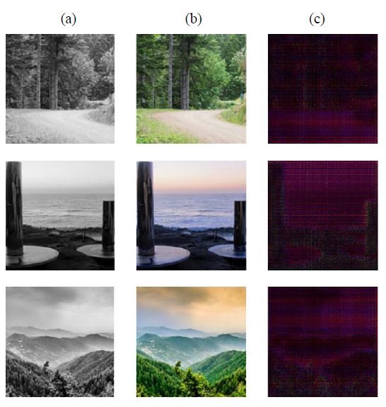
The experiment was conducted by applying the method proposed in this paper with the same data. The output image was largely classified into five categories: sky, plants, sea, ships, and buildings. Before that, the generated image can be seen when the input image was put into the generator in Figure 7.
Sky, plant, sea and building data were available at the following: “kaggle.com/datasets/arnaud58/landscape-pictures” and “kaggle.com/datasets/huseynguliyev/landscape-classification.” Ship data were available at the following: “kaggle.com/datasets/arpitjain007/game-of-deep-learning-ship-datasets.” 12,000 elements of these three data types were properly combined, of which 8,400 were learned and 3,600 were tested.
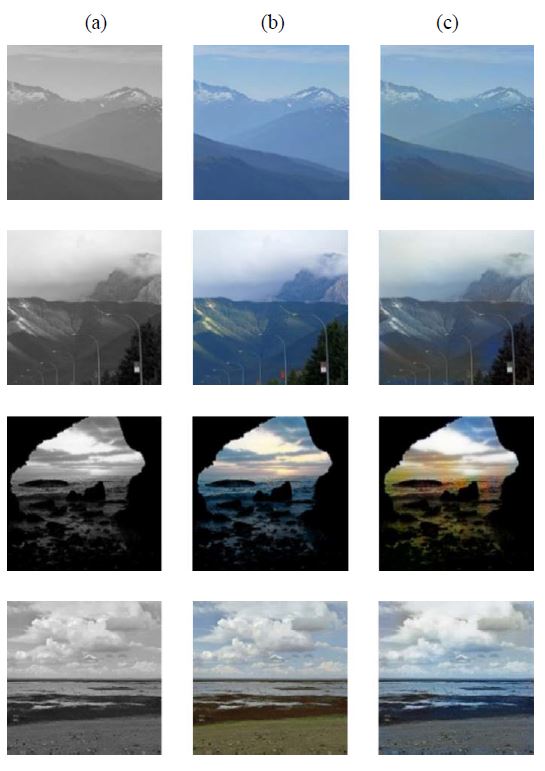
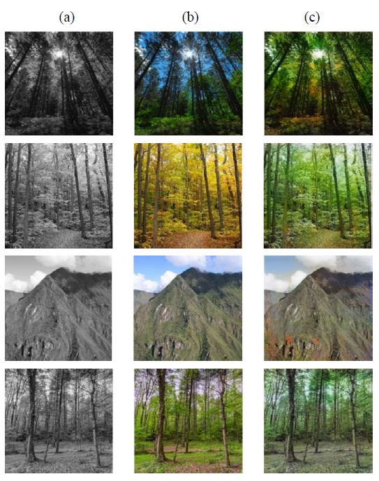
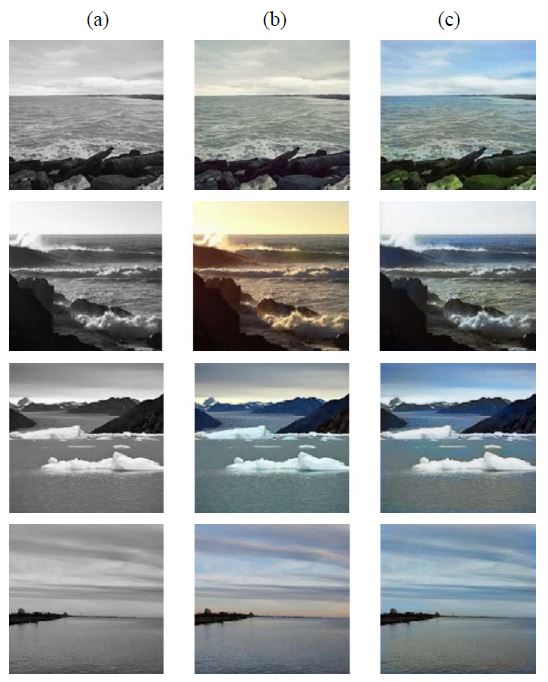
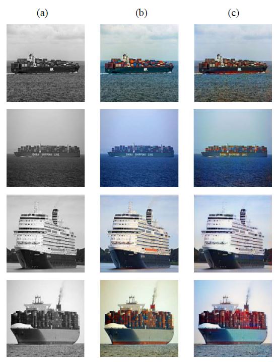
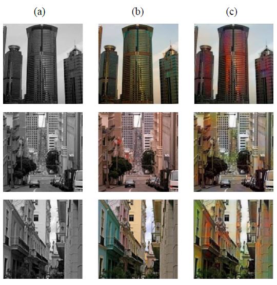
Figure 7 shows the generated images, which contained different types of noises like pink noise and needed improvement. Figures 8 through 12 show the predicted images: sky, plant, sea, ship on the sea, and building, in order. All of the images had a common feature of daytime. First of all, the sky and plant images were heavily affected by the environment such as fog and weather (season). The sea and ship images were for the same reason, and the blue sea made the image itself feel blue as a whole. Lastly, the building was an object that mixed various colors. In all figures, (a) represents the Input images, that is, grayscale images, (b) represents the Ground truth, and (c) represents the color images predicted by applying the proposed method as a Predicted image.
The structural similarity index measure (SSIM) [13] and peak signal-to-noise ratio (PSNR) were evaluated to quantify the colorization quality in this study. The SSIM is a method designed to evaluate human visual image quality differences and similarities, and compares the luminance, contrast, and structure between two images. The PSNR is the noise ratio for the maximum signal that a signal can have. It is a method designed to evaluate loss information for the generated image. The average values extracted between the Ground truth and Predicted image measured 92.68 for the SSIM and 32.73 [db] for the PSNR. Compared with [14][15], it can be seen that the SSIM values were approximately 8% and 4%, and the PSNR was improved by 12 [db] and 8 [db].
In this study, a smooth and clean color image was predicted without other colors invading the boundaries of objects in the image as a whole through the proposed method. In particular, it can be seen that the first image and second image of Figure 9, the second image of Figure 10, and the first image and second image of Figure 11 were colored more naturally with their original colors that Ground truth.
5. Conclusion
Colorizing images is a deeply fascinating problem. In this study, grayscale images were converted into color images through the proposed method by inputting a day landscape that can be seen in everyday life. Our model verifies that it is suitable for automatic image colorization compared with previous studies [16]-[18]. Although it is not completely consistent with the Ground truth and Predicted image, it estimates any color and shows lively colorized images. Moreover, excellent results were shown through the SSIM and SPNR, which are representative image quality measurement methods.
However, the artifact image extracted relatively disappointing results as shown in Figure 12. This is presumed to be owing to a relative lack of training data for the artifact image, so future plans will collect and experiment with a larger amount of data. Also, more accurate colorization is performed on the common pixel values that occupy most of the images. The improves the overall image quality, but the colorization is sometimes not accurate for rare pixel values. We will study areas that classify more clearly in consideration of the concentration of a specific pixel and improve the degraded image quality as a result of extracting various processes.
Author Contributions
Conceptualization & Writing-Original Draft Preparation & Validation & Software, C. R. Park; Methodology & Visualization, C. R. Park and J. H. Kim; Formal Analysis & Re-view & Editing, J. H. Kim; Supervision, S. J. Cho.
References
-
H. Bahng, S. Yoo, W. Cho, D. Keetae Park, Z. Wu, X. Ma, and J. Choo. “Coloring with words: Guiding image colorization through text-based palette generation,” In Proceedings of the European conference on Computer Vision (ECCV), pp. 443-459, 2018.
[https://doi.org/10.1007/978-3-030-01258-8_27]

- F. Baldassarre, D. G. Morín, and L. Rodés-Guirao, “Deep koalarization: Image colorization using CNN and inception-ResNet-v2,” arXiv preprint arXiv:1712.03400, , 2017.
-
S. Iizuka, E. Simo-Serra, and H. Ishikawa, “Let there be color!: Joint end-to-end learning of global and local image priors for automatic image colorization with simultaneous classification,” ACM Transaction on Graphics (Proceedings of SIGGRAPH), vol. 35, no. 4, pp. 1-11, 2016.
[https://doi.org/10.1145/2897824.2925974]

-
G. Larsson, M. Maire, and G. Shakhnarovich, “Learning representations for automatic colorization,” In European Conference on Computer Vision 2016, pp. 577-593, 2016.
[https://doi.org/10.1007/978-3-319-46493-0_35]

-
Z. Yu, Q. Xiang, J. Meng, C. Kou, Q. Ren, and Y. Lu, “Retinal image synthesis from multiple-landmarks input with generative adversarial networks,” Biomed Engineering Online, vol. 18, 2019.
[https://doi.org/10.1186/s12938-019-0682-x]

-
I. Goodfellow, J. Pouget-Abadie, M. Mirza, B. Xu, D. Warde-Farley, S. Ozair, A. Courville, and Y. Bengio, “Generative adversarial networks,” vol. 63, no. 11, pp. 139-144, 2020.
[https://doi.org/10.1145/3422622]

- I. J. Goodfellow, and et al, “Generative adversarial networks,” In Proceedings of the international conference on neural information processing systems (NIPS 2014), vol. 3, pp. 2672-2680, 2014.
- A. Radford, L. Metz, and S. Chintala, “Unsupervised representation learning with deep convolutional generative adversarial networks,” arXiv preprint arXiv:1511.06434, 2015.
- M. Mirza and S. Osindero, “Conditional generative adversarial nets,” Available: https://arxiv.org/abs/1411.1784
-
K. Armanious, C. Jiang, M. Fischer, and et al., “MedGAN: medical image translation using GANs,” Computerized Medical Imaging Graphics, vol. 79, 2020.
[https://doi.org/10.1016/j.compmedimag.2019.101684]

-
P. Isola, J. Y. Zhu, T. Zhou, and A. A. Efros, “Image-to-image translation with conditional adversarial networks,” pp. 1125-1134, 2017.
[https://doi.org/10.1109/CVPR.2017.632]

-
O. Ronneberger, P. Fischer, and R. Brox, “U-Net: Convolutional networks for biomedical image segmentation,” Medical Image Computing and Computer-Assisted Intervention – MICCAI 2015, pp. 234-241, 2015.
[https://doi.org/10.1007/978-3-319-24574-4_28]

-
Z. Wang, A. C. Bovik, H. R. Sheikh, and E. P. Simoncelli, “Image quality assessment: From error visibility to structural similarity,” IEEE Transaction on Image Processing, vol. 13, no. 4, pp. 600-612, 2004.
[https://doi.org/10.1109/TIP.2003.819861]

-
S. Treneska, E. Zdravevski, I. M. Pires, P. Lameski, and S. Gievska, “GAN-based image colorization for self-supervised visual feature learning,” Sensors, vol. 22, no. 4, p. 1599, 2022.
[https://doi.org/10.3390/s22041599]

- J. Zhang, C. Xu, J. Li, Y. Han, Y. Wang, Y. Tai, and Y. Liu, “SCSNet: An efficient paradigm for learning simultaneously image colorization and super-resolution,” Computer Vision and Pattern Recognition, arXiv:2201.04364, , 2022.
-
M. R. Joshi, L. Nkenyereye, G. P. Joshi, S. M. R. Islam, M. Abdullah-Al-Wadud, and S. Shrestha, “Auto-colorization of historical images using deep convolutional neural networks,” Mathematics, vol. 8, no. 12, p. 2258, 2020.
[https://doi.org/10.3390/math8122258]

- F. Baldassarre, D. G. Morín, and L. Rodés-Guirao, “Deep koalarization: Image colorization using CNNs and inception-resnet-v2,” KTH Royal Institute of Technology, 2017.
- M. Agrawal and K. Sawhney, “Exploring convolutional neural networks for automatic image colorization,” Computer Science, 2016. Available: http://cs231n.stanford.edu/reports/2017/pdfs/409.pdf, .

