Decision of complementary filter coefficient through real-time error analysis for attitude estimation using an IMU

Copyright © The Korean Society of Marine Engineering
This is an Open Access article distributed under the terms of the Creative Commons Attribution Non-Commercial License (http://creativecommons.org/licenses/by-nc/3.0), which permits unrestricted non-commercial use, distribution, and reproduction in any medium, provided the original work is properly cited.
Abstract
This paper proposes a method for estimating the attitude (roll and pitch angles) of an inertial measurement unit (IMU) by updating the coefficient of the complementary filter in real time. The complementary filter fuses the data of accelerometer and gyroscope using the coefficient that can compensate the shortcomings occurring when used respectively. The proposed method determines a proper coefficient through analyzing the attitude error in real time. Specifically, the time constant of the filter, related to the coefficient, is determined by the time spent for the gyroscope error exceeds the root mean square (RMS) of the attitude calculated with accelerometer output. We conducted off-line analyses with experimental data to verify the performance of the proposed time-varying complementary filter.
Keywords:
Inertial measurement unit, Complementary filter, Filter coefficient, Error analysis, Attitude estimation1. Introduction
An inertial measurement unit (IMU) consists of accelerometer and gyroscope. The IMU is mainly used to measure the position and attitude of an object. It calculates the changes of the attitude from the initial state using the angular velocity outputs from gyroscope and calculates the position change and linear velocity using the acceleration outputs from accelerometer. However, the difference between the actual states and calculated states increases gradually during calculation. The main cause is an error accumulated while integrating the accelerometer and gyroscope outputs. Thus, such an error is required to be addressed to use the the IMU appropriately.
Various studies on error, which causes the performance degradation of the IMU, have been conducted. Park et al. [1], Flenniken et al. [2] and Yu et al. [3] presented the output model of an IMU with error components and analyzed their effect on the calculated states. Looney [4] presented the effect of linear vibrations caused by the inherent noise of the IMU. Park et al. [5] presented the effect of the output noise on calculated attitude. To improve the reliability and accuracy of the calculated states, two methods can be considered: one is to directly compensate the error components [4][6] and the other is to estimate the states.
Kalman filter [7]-[9] and complementary filter [10]-[12] are most widely used to estimate the states by fusing the outputs of sensors whose performance are determined by coefficients. However, the coefficients are usually fixed and it is inefficient when the characteristics of the motion to estimate changes irregularly. Various studies have been conducted to improve the performance of the filters. Lee [8] and Widodo et al. [9] presented adaptive estimation methods using Kalman filter with compensating external acceleration caused by the change of motion. Song et al. [11] and Yoo et al. [12] presented an adaptive decision method of cut-off frequency for complementary filter based on the pre-analysis about the motion. However, the previously proposed methods of designing time-varying complementary filters require a pre-analysis step to subdivide the motion and inspect their characteristics to prepare appropriate coefficients, while adaptive Kalman filters can be applied without much setup.
In this paper, we propose a method of deciding the coefficient of the complementary filter adaptively only with simple pre-analysis on the error performance of the IMU. In Section 2, we first look into the output of the IMU and investigate the effect of the noise on the attitude calculation. Section 3 introduces the method of updating the complementary filter coefficient using the characteristics of the output that changes according to the motion of the IMU. Finally, the estimation performance of the proposed method is verified using experimental data in Section 4.
2. Sensor Noise and its Effect to Attitude
The output of the sensor contains not only the true value but also the error component. Usually, the output of the sensor can be expressed as follows:
| (1) |
| (2) |
where, So is the measured value, St is the true value of the measuring state, Sb is the bias, and Sr is the inherent random noise. Major factors that contribute to the bias include deterministic component Sd due to installation error, and scale factor component Ss due to the non-linear fit ratio of the output to the input over the operating temperature range. Here, the random noise Sr is assumed to be a white Gaussian noise.

Definition of the coordinate systems and the attitude
When checking the outputs of the IMU in horizontal and stationary state for a sufficient time, the expected averages for the outputs of the accelerometer are 0 for X and Y axes, g (gravitational constant) for Z axis, and 0 for all three axes for the outputs of the gyroscope. If the average is different from the expected value, the difference can be considered to be a bias. However, the temperature of the sensor is constant and the output of the sensor in pre-analysis step can be compared to the actual use step, the bias component can be ignored.
The roll and pitch angles using the outputs of the IMU can be calculated by the following equations.
| (3) |
| (4) |
| (5) |
| (6) |
Here, , and are the outputs of the accelerometer for each axis, ϕA and θA are the roll and pitch angles calculated using the accelerometer outputs, and are the outputs of the gyroscope for each axis, and ϕG and θG are the roll and pitch angles calculated using gyroscope outputs.
Since there exists the random noise in the outputs of the IMU, the actual outputs of the accelerometer and the gyroscope can be expressed as follows:
| (7) |
| (8) |
where, Δt denotes the sample time, denotes the true value and Δ( ∙ ) denotes the random noise component of the output. If the random noise is included in the outputs, the calculated roll and pitch angles can be rewritten as follows [5]:
| (9) |
| (10) |
| (11) |
| (12) |
3. Time-Varying Complementary Filter
3.1 Conventional complementary filter
When calculating attitude with the outputs of the accelerometer, the results show a large deviation occur by the high frequency band noise while there is drift phenomenon due to the low frequency band noise in case of the gyroscope. Complementary filter, which can be implemented simply through combining the low-pass filter (LPH) and high-pass filter (HPF) as shown in Figure 2, is widely used to compensate these shortcomings of the two sensors and estimate the reliable attitude.

Flowchart of the conventional complementary filter
In Figure 2, is the low-pass filtered attitude calculated using the output of the accelerometer θA and is the high-pass filtered attitude calculated using the output of the gyroscope θG. θC is an estimated attitude by fusing and . The LPF removes the high frequency noise in θA resulting has small deviation than θA and the HPF removes the low frequency band noise of θG so that the drift phenomenon appears less in than θG. The transfer function of the complementary filter shown in Figure 2 is given by
| (13) |
where, τ is time constant that determines the operation of the filters. Equation (13) can also be expressed by Equation (14) in the time domain. Here, α is the filter coefficient and represents the fusion ratio of θA and .
| (14) |
Meanwhile, the relationship between the time constant τ and the cut-off frequency fcutoff of the filters is as follows:
| (15) |
In the point of view of frequency, the output of the LPF has a lower frequency band than fcutoff, and the output of the HPF has a higher frequency band than fcutoff. Therefore, fcutoff can be regarded as the intersection of reliability between HPF and LPF. From this, it can be derived that time constant τ also represent the intersection of reliability.
On the other hand, in the point of view of error performance, if drift is smaller than ΔθA, it can be said that θG is more reliable than θA. This leads to the conclusion that HPF, filtering θG, is more reliable than LPF, filtering θA. However, if drift exceeds ΔθA, the reliability is reversed, making LPF more reliable than HPF. Thus, the point where drift became equal to ΔθA can be considered as an intersection of reliability between LPF and HPF, and the time spent can be used as τ for the filter coefficient.
3.2 Relation between Random Noise and RMS
Random noise of the accelerometer output can be calculated by the following Equation (16) [4][6]. For this study, MTi-670 (XSens) IMU was used, and the specifications of the built-in accelerometer is given in Table 1. In this case, the calculated result is 0.0132m/s2.

Specifications of the accelerometer of MTi-670
| (16) |
Usually, Δab is close to the root mean square (RMS) of the output at a stationary state. RMS is calculated by
| (17) |
where, xi is the measured value, is the expected value, and N is the size of the sample.
Figures 3 and 4 compare Δab with and ΔθA with θARMS, respectively, where the IMU is stationary. ΔθA is calculated by substituting Δab into Equation (9). The calculated result is 0.0763°. It appears that Δaband ΔθA are similar to the RMS of each data when the averages of ab and θA are taken as the expected value. The calculated RMSs are 0.0111 m/s2 and 0.0650°.

Accelerometer outputs in stationary state (X-axis)

Pitch angle in stationary state
In the motional state, it is hard to define Δab and ΔθA accurately as the ratio of the motional component from the accelerometer output and the attitude increases and the effect of the noise decreases relatively. However, they can be presumed by the similarity of the random noise and RMS in the stationary state, that is, Δab and ΔθA in the motional state can be replaced with their RMS respectively. Even if the changes of the sensor output and attitude are irregular, calculating the RMS for short periods of time continuously will be same with calculating as if there is very little changes, and the results can be approximate values of Δab and ΔθA.
Figures 5 and 6 show that the successively calculated RMS for short period of time (N = 10 in this case) of ab and θA are similar to those of calculating results for overall data in stationary state. Here, the moving averages of ab and θA were used as expected values when calculating each RMS. Therefore, it may be inferred that the characteristics of RMS are also similar in motional state. Thus, we propose a method of updating the coefficient of the complementary filter using the time spent for θG to exceed the error range of θA, based on RMS, as a time constant τ.

Comparison of RMS (X-axis)

Comparison of RMS (pitch angle)
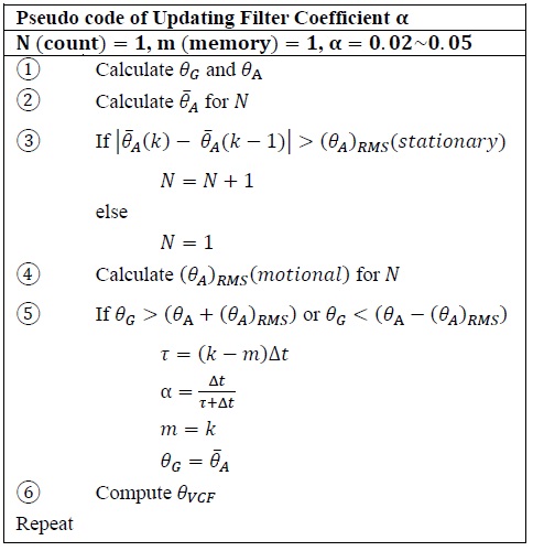
Table 2 shows the process of the proposed method. Firstly, calculate the attitudes θG and θA using outputs of the IMU, and then calculate the moving average of θA. If the difference between the current sample time k and the previous sample time (k − 1) of the moving average is greater than the RMS in a steady state, which is acquired in pre-analysis step, recognize as the IMU is in a motional state and increases the count N, if not, it will be initialized. While the motion is recognized continuing, the RMS of the attitude is calculated using the moving average as an expected value with reference to the increasing N, and use it as an attitude error. When the θG exceeds the RMS range of the θA, update the filter coefficient using the time spent from previous update, memorize the currently updating sample time to use in next update, and initialize θG with to remove excessive drift. Finally, the attitude θVCF is estimated. The initial value of the coefficient, before the initial update, can be selected as a commonly used value between 0.02 and 0.05.
Algorithm for filter coefficient update
4. Performance Verification
The complementary filter, designed with proposed method, was implemented through Matlab to verify the estimation performance. To confirm that the coefficient α is updated properly regardless of the motion of the IMU, the data that the attitudes change randomly was used for the simulation as shown in Figure 7.

Pitch angles in motional state
Figure 8 shows the change in sample size recognized that IMU is continuing its motion due to the difference between moving average, compared to the attitude error in stationary state, of the attitude in sample time.

Recognition of the motion
Figure 9 compares the drift of θG and error range of θA and shows coefficient change correspondingly. Since θG is initialized with , calculated for N shown in Figure 8, at the intersections, reliability for θG and θA become almost same, so α appears as near 0.5 at that point. As the motion continues after the coefficient update, θG gradually loses its reliability due to drift, while reliability of θA relatively increases. It can be seen that α converges to values between 0.02 and 0.05 when the motion is prolonged, which are commonly used coefficients in conventional complementary filter.

Change of filter coefficient according to the motion
Figure 10 shows the adjusted θG. As the drift is removed, compared to that shown in Figure 7, it does not deviate from the error range of θA.

Change of error range due to motion
In Figure 11 and 12, pitch angle estimated through varying complementary filter (VCF) designed with the proposed method is compared to that estimated with conventional complementary filter (CCF) whose coefficients are fixed as 0.02 and 0.05. Also, attitude errors with reference to the pitch angle from the IMU are compared. Figure 11 shows that VCF has better estimation performance than CCF with a coefficient of 0.02 when the direction of motion changes or attitude changes rapidly within a short period of time. However, for motion with small attitude changes without changing the direction, it shows relatively inferior performance compared to CCF. Still, the degree of superior performance is overwhelming compared to the degree of inferior performance. Figure 12 shows the performance comparison of VCF with CCF whose coefficient has increased to 0.05. As the influence of the accelerometer in the CCF increased, the deviation of the estimation result increased, so that the difference in estimation performance of CCF and VCF in the part where attitude change is small has decreased accordingly. On the other hand, as the influence of the gyroscope in CCF decreased, which means that the effect of drift also decreased, the difference in estimation performance of two filters has decreased in the part where attitude change large as a result.

Comparison of attitudes in motional state (α = 0.02)

Comparison of attitudes in motional state (α = 0.05)
From these results, it was confirmed that the CCF can expect appropriate performance by carefully selecting coefficient for motion to be estimated, but if the movements are diverse, the performance will inevitably be focused on one side, either small or large motion. In addition, it was confirmed that the estimation error of CCF was not relatively close to zero compared to the estimation error of VCF. These means that unless the step of accurate measurement and correction of drift is included in the estimation process of the CCF, the estimated result are inevitably affected and the performance is degraded. As a result, it was confirmed that the VCF proposed in this paper is free from the coefficient-dependent problem of CCF and can appropriately estimate the attitude of the IMU that move arbitrarily and irregularly by updating coefficient in real time through simple error analysis without complicated pre-analysis step.
5. Conclusion
This paper proposed a coefficient update algorithm for a complementary filter. The proposed algorithm analyzes attitude error changing in real time and determines the appropriate coefficient for the current motion. The results of this study can be summarized as follows:
- (1) Analyzed the relationship between the calculated posture error and RMS using the output of the accelerometer.
- (2) Designed the method for recognizing the motion state.
- (3) Defined the method of updating the coefficient of the complementary filter using time spent that the attitude calculated using the gyroscope output exceeds the error range of the attitude calculated using the accelerometer output.
- (4) Verified the validity of the proposed method through offline analysis using experimental data.
Our future work will involve an improvement on recognizing that the motion continues based on precise analysis for error characteristics of the IMU. Also, real application of the proposed method on vehicle will be involved.
Acknowledgments
This research was supported by Institute of Civil Military Technology Cooperation (ICMTC) of Agency for Defense Development (ADD), South Korea. (Project No.: 15-CM-SS-01, Project Title: Development of Towed Interferometric Synthetic Aperture Sonar (InSAS))
Author Contributions
Conceptualization, S. -J. Chon and J. -H. Kim; Methodology, S. -J. Chon and J. -K. Choi; Validation, S. -J. Chon and J. -K. Choi; Writing—Original Draft Preparation, S. -J. Chon; Writing—Review & Editing, S. -J. Chon, J. -K. Choi and J. -H. Kim; Supervision, J. -K. Choi and J. -H. Kim.
References
-
M. H. Park, Y. Gao, “Error and performance analysis of MEMS-based inertial sensors with a low-cost GPS receiver,” Sensors, vol. 8, pp. 2240-2261, 2008.
[https://doi.org/10.3390/s8042240]

- W. S. Flenniken, J. H. Wall, and D. M. Bevly, “Characterization of various IMU error sources and the effect on navigation performance,” ION GNSS, 2005.
- H. S. Yu, T. H. Kim. C. J. Kim, Y. S. Lee, and H. W. Park, “A study on methods of measuring and compensating misalignment between inertial sensor body and housing frame,” Journal of the Korea Institute of Military Science and Technology, vol. 17, no. 1, pp. 135-141, 2014.
- M. Looney, Anticipating and Managing Critical Noise Sources in MEMS Gyroscopes, https://www.analog.com/en/technical-articles/critical-noise-sources-mems-gyroscopes.html, , Accessed March 11, 2021.
- C. G. Park, K. J. Kim, H. W. Park, and J. G. Lee, “Development of an initial coarse alignment algorithm for strapdown inertial navigation system,” Journal of Institute of Control, Robotics and Systems, vol. 4, no. 5, pp. 674-479, 1998.
- A. Fan, How to Improve the Accuracy of Inclination Measurement Using an Accelerometer, https://www.analog.com/en/analog-dialogue/articles/how-to-improve-the-accuracy-of-inclination-measurement-using-an-accelerometer.html, , Accessed March 14, 2021.
-
M. J. Choi and J. K. Lee, “IMU-based attitude estimation Kalman filter with kinematic constraint projection,” Journal of Institute of Control, Robotics and Systems, vol. 24, no. 2, pp. 175-181, 2018.
[https://doi.org/10.5302/J.ICROS.2018.17.0204]
-
J. K. Lee, “Comparison of acceleration-compensating mechanisms for improvement of IMU-based orientation determination,” Transaction of the Korean Society of Mechanical Engineers-A, vol. 40, no. 9, pp. 783-790, 2016.
[https://doi.org/10.3795/KSME-A.2016.40.9.783]
-
R. B. Widodo and C. Wada, “Attitude estimation using ualman filtering: External acceleration compensation considerations,” Journal of Sensors, vol. 10, pp. 10-24, 2016.
[https://doi.org/10.1155/2016/6943040]
-
H. G. Min, J. H. Yoon, J. H. Kim, S. H. Kwon, and E. T. Jeung, “Design of complementary filter using least square method,” Journal of Institute of Control, Robotics and Systems, vol. 17, no. 2, pp. 125-130, 2011.
[https://doi.org/10.5302/J.ICROS.2011.17.2.125]
-
S. K. Song, H. S. Woo and K. C. Kong, “Estimation of tibia angle through time-varying complementary filtering and gait phase detection,” Journal of Institude of Control, Robotics and Systems, vol. 21, no. 10, pp. 944-950, 2015.
[https://doi.org/10.5302/J.ICROS.2015.14.0122]
-
T. S. Yoo, S. K. Hong, H. M. Yoon and S. S. Park, “Gain-scheduled complementary filter design for a MEMS based attitude and heading reference system,” Sensors, vol. 11, no. 4, pp. 3816-3830, 2011.
[https://doi.org/10.3390/s110403816]