Characteristics of the plume formed by the buoyant discharges from the river

1. Introduction

The buoyant discharges from the river into the ambient coastal region make a transition from jet to surface plume forming two-layer structure in the ambient sea.

Freshwater discharges produce pressure gradients by density anormalies which are important forcing term that can drive circulation in the ambient sea.

The pattern of buoyant water discharge varies according to the characteristics of the ambient coastal region such as geometrical constraints of coastal configuration and bottom topography, wind stress, ambient coastal current, the amount of buoyant discharges and Coriolis force acting upon the outflow, etc. In other words, the analysis of buoyant discharges from the river into the ambient coastal region is so much complicated by many factors that it is more clear to deal the influence of each factor seperately rather than to describe all the variabilities.

The spreading of buoyant river water discharge into the ambient sea is the case in which a light rotating fluid spreads over a heavier fluid. The main features are the formation of a density current by lateral boundaries, formation and dissipation of the front, formation of eddy structures etc.

Kao and Pao [1] conducted numerical analysis on the buoyant surface discharge into an ambient body of water using a two-dimensional model. The results showed the establishment of a surface density current with the strong surface convergence and downwelling near the front. Stern et al. [2] showed from the laboratory experiment that light rotating fluid spreading over heavier fluid in the vicinity of a vertical wall forms a boundary jet and a certain fraction of the boundary transport is not carried by the nose but seperates from the coast and an intermittent boundary current forms. The results showed the stability condition of buoyancy-driven coastal currents.

The stability of buoyancy-driven coastal currents were experimented by Griffiths et al. [3] in the laboratory. The current became unstable to nonaxisymmetric disturbances with the continuous release of fluid from the source. It was showed that the wavelength and phase velocities of the disturbances are consistent with the model of baroclinic instability of two-layer flow. They pointed out that when the current only occupies a small fraction of the total depth, barotropic processes can also be important with the growing waves gaining energy from the horizontal shear. This study explained the stability of buoyancy-driven coastal currents by frictional dissipation due to Ekman layers and horizontal shear. But for the stability of buoyancy-driven coastal currents, the factors such as the bottom topography configuration and interfacial friction between upper warm surface water and ambient sea water below are also thought to be important so that more detailed analysis is needed for these factors.

The spreading of light rotating fluids into the ambient sea deviates to the right in the Northern Hemisphere by the Coriolis force. But the direction of the spreading is affected by many factors which include not only Coriolis force but also bottom and interfacial frictions, geometrical constraints, etc. Takano [4][5] predicted that the outflow of river water deviates to the right in the Northern Hemisphere with the extent of deviation being dependent on the parameter R₀, given as R₀ = fW/A_h where f is the Coriolis parameter, W is a width of the mouth of the estuary and Ah is the horizontal eddy viscosity coefficient. But Zhang et al. [6] pointed out that Takano’s solution requires values of A_h about two orders of magnitude higher than values of real fields and that this discrepancy suggests that neglected processes such as entrainment or interfacial friction may be significant. Nof [7] examined the dynamics of outflows from sea straits and wide estuaries using frictionless single and two-layer model. The single layer model predicted that an outflow from the estuary deflects to the right or left depending upon the depth of the basin into which it debouches. The two-layer model predicted spreading direction of an outflow depends upon the vorticity formed during an outflow such that negative vorticity approximately equal to or larger than Coriolis parameter makes an outflow deflect to the left. These results suggested the important role of Coriolis force, interfacial friction and bottom topography on the spreading direction of the light rotating fluid into the ambient sea.

The goal of this study is to analyse the buoyant discharges from the river into the ambient coastal region attempting especially for the following questions to clarify.

(a) How does the buoyant discharges form the surface plume and buoyancy-driven density current?

(b) What is the condition for the stability of the buoyancy-driven density current?

(c) What is the factors that control the direction of spreading of buoyant discharges?

The above mentioned questions are attempted to solve using the two-layer numerical model including Coriolis acceleration, bottom stress, interfacial friction and entrainment processes. To analyse more systematically, governing equations are non-dimensionalized using appropriate scales for the variables. Some non-dimensional numbers such as Froude, densimetric Froude and Kelvin numbers are obtained and some characteristic scales are defined as a result of non-dimensionalization. These numbers and scales are controlling factors in the dynamics of warm water discharge. Varying these numbers and scales, above mentioned questions are examined and discussed.

2. Model Description

We consider two-layer fluid system in which the motion is generated by the input of effluents from the source of width W located at the center of the left side wall; see Figure 1. Densities and initial thickness of upper layer are ρ₁ = λρ₀ and H₁ while those of lower layer are ρ₁ and H₂ respectively. Details are shown in Figure 2. with the coordinate system. Here λ is the ratio of the densities of two layer, i.e., λ = ρ₁/ρ₀. Thickness of each layer is varied with the motion by the surface and interfacial displacement η₁, and η₂ respectively, i.e.,

Figure 1:

Upper view of the model. W denotes source width. Thick line is closed boundary and thin line is open boundary.

Figure 2:

Side view of the model.

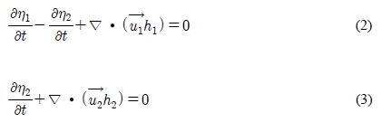
where h₁ and h₂ are upper and lower layer thickness. Hereafter the suffix 1, 2 denotes upper and lower layer respectively. Under the hydrostatic approximation, the layer averaged incompressible continuity equations for each layer can be written as

Here 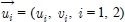is the velocity vector where u_i, ν_i are x and y component velocities respectively. The momentum equations for each layer are as follows;

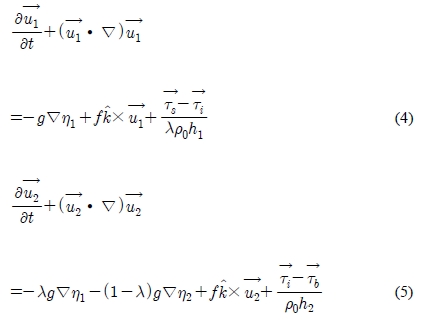
Here g is the gravitational acceleration; f is the Coriolis parameter; are the surface, interfacial, bottom stresses respectively. and are parametrized by

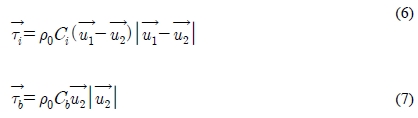
where C_i, and C_b are interfacial and bottom friction coefficients, respectively.

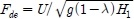
Initially, ambient water is motionless except at the source where effluents are discharged at the rate Q so that the velocity is U = Q/WH₁. At solid boundaries, normal component of velocities is zero while at open boundary, free radiation conditions are applied for each layer as follows.

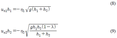
where u_n1, u_n2 are velocity components perpendicular to the open boundary for upper and lower layer respectively.

Introducing scales for horizontal length as source width W, velocity as source discharge velocity U , time as T = W/U, non-dimensional variables are defined as . Substituting these in the governing equations, non-dimensional governing equations can be obtained revealing five controlling dimensionless parameters; R_i = C_iW/H₁, the scale of interfacial friction; R_b = C_bW/H₁, the scale of bottom friction; R_k = fW/U, the Kelvin number, the ratio of the imposed geometric scale W to the intrinsic scale of internal radius of deformation, reflecting the importance of the Coriolis effect in the dynamics; , the Froude number, representing the ratio of inertial force to gravity force; and , the densimetric Froude number, the ratio of inertial force to buoyancy force. Non-dimensional governing equations are then

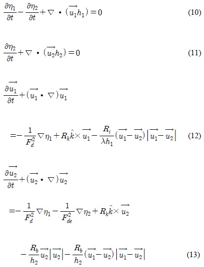
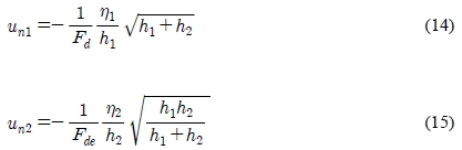
Here the primes are omitted to simplify the notation. Non-dimensional boundary conditions for the open boundary are

A finite difference scheme was used for the numerical solution, where forward differences for the time derivatives, centered differences for the space derivatives and four point averaging method for Coriolis terms are used and solutions are obtained explicitly. Grid spacing and time interval are set as ∆x = ∆y = ∆S = 1.0 and ∆t= 0.01 satisfying the CFL stability condition of which C∆t/ ∆S ≤ 1 where being the deepest depth. Number of grids are set as i = 50, j = 80 in the x, y directions respectively.

3. Results and Discussion

Numerical experiments are conducted varying the non-dimensional parameters and bottom topography. Details of the experiments are presented in Table 1. The configurations of bottom topography denoted by B1, B2 and B3 in Table 1 are shown in Figure 3. Experiment 1 (hereafter denoted by Exp. 1) is the basic experiment which will be compared with other experiment. In Exp. 1, parameters configured are λ = 0.99, R_k = 0.1, F_d = 0.1, F_de = 0.1, R_i = 0.1, R_b = 0.1 and bottom topography is same depth (B1). Results are analyzed focusing to the propagation of the plume, effects of non-dimensional parameters on the flow characteristics of the plume, and effects of bottom slope.

Table 1:

Conditions of the various experiments.

Figure 3:

Bottom configurations. B1 denotes flat bottom, B2 downward slope and B3 upward slope.

3.1 Propagation of the plume

Buoyant discharges front the river eventually become the surface plume spreading over the ambient coastal sea. It is usually known that because of Coriolis effect, the plume turns to the right as seen to the spreading direction in the northern hemisphere. But besides the Coriolis effect, the factors that control the spreading of the plume include many factors.

Development of the plume with time for the basic experiment (Exp. 1) is presented in Figure 4(a), (b). Figure 4(a), (b) represents the distribution of the velocity field and contours of the interfacial displacement with time t = 90, 180, 270, 360, 450 and 540, respectively. Dotted lines of the Figure 4 (b) represent negative value, i.e, penetration to the lower layer. For the flat bottom case of Exp. 1, by the Coriolis effect (O’Donnel [8]), the plume deviates slightly to the right in the direction of the plume propagation (see Figure 4 (a)), and the upper layer of the right side of the plume from the source line becomes deeper while in the left side, it becomes shallower (see Figure 4 (b)). The Coriolis effect also suppress the instability of the velocity field of the upper layer in the right side of the plume (Griffiths et al. [3]), so that it shows somewhat more stable structures than in the left side.

Figure 4:

Development of the plume with time t = 90, 180, 270, 360, 450, 540 for the basic experiment (Exp. 1). (a) Upper layer velocity distribution, (b) Contours of interfacial displacement.

Propagation speed of the plume to the offshore direction was examined by comparing the frontal position with time for the various experiments (Figure 5).

Figure 5:

Propagation of the frontal position with time for various experiment.

Here, experiments compared were chosen to be the representative of the non-dimensional parameters. The frontal position X_f in Figure 5 is defined by the maximum x of u = 0.01 contour. Fast propagation can be achieved by the two cases of small interfacial friction (Exp. 4, R_i = 0.02) and large density difference between upper and lower layers (Exp. 19, λ = 0.5). Front propagations are slowed down with increasing the viscosity effect of two layers and the decrease of horizontal density gradient (Lindon et al. [9]; Noh et al. [10]). Large interfacial friction generates turbulent motion by the viscosity effect so that propagation speed is retarded. Small density difference between upper and lower layer can make similar effect of large viscosity effect. Upper layer plume with large density difference to the lower layer can further go through offshore without mixing with lower layer. Coriolis effect (R_k) inhibit the plume propagation to the offshore as shown in Figure 5. Compared with the basic experiment, bottom friction cannot affect largely on the propagation speed of front. In the small Froude number case, the propagation speed is somewhat faster than the basic experiment. These effects are more discussed in the section.

3.2 Effect of bottom slope

The effect of bottom slope on the spreading of the plume was firstly examined through the Experiment 1, 2 and 3 of Table 1. All experiments were conducted under the same condition except the different bottom topography of B1 (flat bottom) in Exp. 1, B2 (downward slope) in Exp. 2 and B3 (upward slope) in Exp. 3. Figure 6 (a), (b), (c) represent the upper layer velocity distribution and (d), (e), (f) interfacial displacement of Exp. 1, Exp. 2 and Exp. 3 at time t = 540 respectively.

Figure 6:

(a), (b), (c). Upper layer velocity distribution at t = 540 of the experiments for (a) flat bottom, (b) downward slope and (c) upward slope of Exp. 1, 2, and 3. (d), (e), (f). Interfacial displacement at t= 540 of the experiments for (a) flat bottom, (b) downward slope and (c) upward slope of Exp. 1, 2, and 3.

For the single layer fluid, if the bottom gets deeper from the source to the offshore, the total fluid layer increases offshore and hence offshore propagating particles gain the positive relative vorticity by vortex tube stretching resulting in the cyclonic circulation. In the case of two layer fluids, forcing can be decomposed into a baroclinic and barotropic component. Under the purely baroclinic forcing, bottom friction is negligible so that potential vorticity is conserved. In this case, an offshore propagating water parcel gains anticyclonic vorticity due to the vortex tube squashing since the upper layer depth decreases offshore regardless of the bottom slope. The barotropic component can force upper layer fluid through the bottom and interfacial friction terms.

The structures of the buoyant plume are complicated by the above mentioned two components in addition to the Coriolis effect. As shown in Figure 6 (e), from the source to the offshore, the upper layer thickness of right side firstly increases because of the supply from the source and Coriolis effect but soon it decreases because of the buoyancy effect and reduced speed which results in weakening Coriolis effect as farther down from the source. On the other hand, the upper layer thickness of left side firstly decreases by the effect of the Coriolis effect but as farther down to the offshore, it recovers the original thickness because of the weakening of the Coriolis effect. The changes of the upper layer thickness in both sides result in the same effect as increasing layer thickness in the left side and decreasing layer thickness in the right side. Consequently, upper layer fluids of left side experience the vortex tube stretching by which the fluid particles in the layer get the positive vorticity resulting in the cyclonic circulation, while those of right side gain negative vorticity due to the vortex tube squashing resulting in the anticyclonic circulation as shown in Figure 6 (b).

In the offshore fairly far from the source, barotropic forcing becomes main forcing term. Hence the fluid column in the region gains cyclonic vorticity due to the bottom slope so that the plume tends to deviate to the left as a result of the cyclonic circulation as shown in Figure 6 (b). Zhang et al. [6] also showed in their model that in the downward slope of bottom, when 0 < U₂/U₁ < 1, the upper layer plume turns to the left where U₁ and U₂ are upper and lower velocity respectively. The counterclockwise rotating eddies are not formed except near the source region because the formation of eddy is inhibited by the Coriolis effect.

If the bottom becomes shallower, the barotropic forcing becomes more and more strong due to the effect of bottom friction so that particles in the fluid column acquire the negative vorticity inducing the clockwise circulation so that the plume turns to the right with the effect of negative vorticity and Coriolis effect as shown in Figure 6 (c) and 6 (f).

For the case of large Kelvin number of R_k = 0.5, the effect of bottom slope is analysed through experiments 12, 13 and 14 of B1, B2 and B3 bottom topography respectively. Developement of the plume with time is shown for the Exp. 12 of R_k = 0.5 and same depth (B1) is shown in Figure 7 (a), (b), the upper layer velocity distribution and contours of interfacial displacement respectively. Figure 8 (a) represent the upper layer velocity distribution and (d), (e), (f) interfacial displacement of each experiment at time t = 540 respectively. Common features are the formation of the anticyclonic vorticities and boundary currents. For the flat bottom case, as viewed to the offshore, anticyclonic vortexes are produced on the right, while cyclonic vortexes are on the left side as in Figure 8 (a). But for the deepening bottom of B2, the plume bulge is confined near the source region to form the boundary currents both sides as shown in Figure 8 (b). Shallowing bottom of B3 also suppress for the plume to propagate to the offshore but it can produce strong anticyclonic vortex as in Figure 8 (c).

Figure 7:

Development of the plume with time t = 90, 180, 270, 360, 450, 540 for the Rk= 0.5 (Exp. 12). (a) Upper layer velocity distribution, (b) Contours of interfacial displacement.

Figure 8:

(a), (b), (c). Upper layer velocity distribution at t = 540 of the experiments of Rk = 0.5 for (a) flat bottom, (b) downward slope and (c) upward slope of Exp. 12, 13, and 14. (d), (e), (f). Interfacial displacement at t = 540 of the experiments of Rk = 0.5 for (a) flat bottom, (b) downward slope and (c) upward slope of Exp. 12, 13, and 14.

3.3 Effect of bottom Friction

The effect of bottom friction on the plume is examined through the experiment 1, 8, 9, 10 and 11 varying the scale of bottom friction R_b as 0.02, 0.1 and 0.5 for the B1 and B2 bottom topography. Figure 9 and 10 (a), (b) shows the upper layer velocity distribution and contours of interfacial displacement of Exp. 8 and 9 respectively. Large bottom friction makes the plume more turbulent to reduce the propagation speed. Figure 11 (a), (b), (c), (d), (e) and (f) shows the upper layer distribution and interfacial displacement of Exp. 2, 10 and 11 at time t = 540 for the cases of R_b = 0.02, 0.1, 0.5 for B2 bottom topography. Bottom friction helps vertical mixing of momentum and density over the fluid column and diffuses relative vorticity (Munchow et al. [11]). Therefore, as bottom friction becomes weaker, the eddies are more easily formed as a result of stronger relative vorticity. For R_b = 0.02 case of Figure 11 (a), cyclonic eddies on the left side and anticyclonic eddies on the right side of the plume are formed as viewed in the direction of the plume propagation from the source. Left side eddies are the result of positive vorticity acquired by the fluid column as the deepening of bottom. Right side eddies are induced by the Coriolis effect. Near the source, Coriolis effect dominates so that the flow deviates to the right. But as farther down from the source, the effect of bottom topography results in positive vorticity so that the flow turns to the left. As R_b increases, bottom friction diffuses the relative vorticity so that it flattens the eddy-like structures (Chao et al. [12]). Figure 12 shows the distribution of the interfacial displacement along the x-axis of two lines at y = 30, 50 which are the right and left lines from the source line y = 40. The eddies formed by the positive vorticity make the interfacial displacement more upwards at the right side of the plume reducing the upper layer at the left side of the plume. Right side eddies formed by Coriolis effect deepen the interfacial friction. So, for R_b = 0.02, it is deepest both positively and negatively near the source. As R_b increases, eddy-like structures are disappeared, and the plume propagate farther down from the source. Intensive mixing makes the interfacial displacement more deepen both sides positively and negatively so that as father down from the source, interfacial displacement is deepest both positively and negatively for R_b = 0.5.

Figure 9:

Developement of the plume with time t = 90, 180, 270, 360, 450, 540 for the Rb= 0.02 (Exp. 8). (a) Upper layer velocity distribution, (b) Contours of interfacial displacement.

Figure 10:

Developement of the plume with time t = 90, 180, 270, 360, 450, 540 for the Rb = 0.5 (Exp. 9). (a) Upper layer velocity distribution, (b) Contours of interfacial displacement.

Figure 11:

(a), (b), (c). Upper layer velocity distribution at t = 540 of the experiments for the downward slope B2 varying Rb as (a) 0.02 (Exp. 10), (b) 0.1 (Exp. 2) and (c) 0.5 (Exp. 11). (d), (e), (f). Interfacial displacement at t= 540 of the experiments for the downward slope B2 varying Rb as (a) 0.02 (Exp. 10), (b) 0.1 (Exp. 2) and (c) 0.5 (Exp. 11).

Figure 12:

Distribution of the interfacial displacement along the x axis at two lines of y = 30 and 50 for Rb = 0.02 (Exp. 10), 0.1 (Exp. 2) and 0.5 (Exp. 11).

3.4 Effects of Interfacial Friction

The effects of interfacial friction is analyzed through the experiment 2, 4, 5, 6, 7 and 8 varying the scale of the interfacial friction R_i as 0.02, 0.5 and 0.1 for the B1 and B2 bottom topography. Developement of the plume with time for Exp. 4 ( R_i = 0.02, B1) and Exp. 5 (R_i = 0.5, B1) are presented in Figure 13 and 14 (a), (b), the distribution of the velocity field and contours of the interfacial displacement with time t = 90, 180, 270, 360, 450 and 540, respectively. The plume becomes remarkably unstable and eddies of right and left side as viewed from the source to offshore vividly develope in the case of small interfacial friction. The propagation speed is much faster in the small interfacial friction. Viscous effect between the two layers generates turbulence and results in mixing between the two layers so that the formation of eddies is inhibited and propagation speed reduces. Most remarkable feature of the small interfacial friction is the formation of the left side boundary current. As shown in Figure 13 (b), the small negative vortex is generated and this vortex grows and propagates along the left side boundary as viewed from the source to the offshore. This vortex gets larger with the supply of energy from the interactions of main eddies which can maintain the left side boundary current. Figure 15 (a), (b), (c) represent the upper layer velocity distribution and (d), (e), (f) interfacial displacement of each experiment at time t = 540. Interfacial friction inhibits the baroclinicity of the flow. The weaker interfacial friction makes the upper and lower layer more distinguishable. The thickness of the upper layer decreases as farther down from the source so that the upper layer fluid aquires anticyclonic vorticity as shown in Figure 15 (a) of the weakest value of R_i = 0.02.

As R_i increases, vortices are diffused so that the effect of bottom topography dominates to produce the cyclonic voticity as shown in Figure 15 (b) and 15(c).

Figure 13:

Developement of the plume with time t = 90, 180, 270, 360, 450, 540 for the Ri = 0.02 (Exp. 4). (a) Upper layer velocity distribution, (b) Contours of interfacial displacement

Figure 14:

Developement of the plume with time t = 90, 180, 270, 360, 450, 540 for the Ri = 0.5 (Exp. 5). (a) Upper layer velocity distribution, (b) Contours of interfacial displacement.

Figure 15:

(a), (b), (c). Upper layer velocity distribution at t = 540 of the experiments for the downward slope B2 varying Ri as (a) 0.02 (Exp. 6), (b) 0.1 (Exp. 2) and (c) 0.5 (Exp. 7). (d), (e), (f). Interfacial displacement at t = 540 of the experiments for the downward slope B2 varying Rb as (a) 0.02 (Exp. 10), (b) 0.1 (Exp. 2) and (c) 0.5 (Exp. 11).

3.5 Effects of Froude Number

Experiments were conducted by varying the Froude number as 0.05 (Exp. 17, 18), 0.1 (Exp. 1), 0.2 (Exp. 15, 16). Developement of the plume with time for Exp. 15 (F_d = 0.2, B1) and Exp. 17 (F_d = 0.05, B1) are presented in Figure 16 and 17(a), (b), the distribution of the velocity field and contours of the interfacial displacement with time t = 90, 180, 270, 360, 450 and 540, respectively. Typical feature of the effect of Froude number is the wave-like disturbances occur at high Froude number as shown in Figure 16. Griffiths et al. [3] suggested that critical value of Froude number exists at which density current becomes unstable and forms wave-like feature. As shown in Figure 16 (b), eddies in the right side as viewed from the source to offshore develope with time which eventually becomes large eddy while in the left side, small eddy is firstly generated and this eddy grows larger to propagate to the offshore direction. Left side velocity distributions show very complicated features while those of right side show only eddy-like feature which is the result of the Coriolis effect. For the case of low Froude number, eddies are rarely generated as shown in Figure 17. But Froude number effect is closely related with the Kelvin number effect because both number contains the horizontal velocity and geometry scale. If R_k increases, the effect is the same as the increasing the Froude number. Figure 18 (a), (b) shows the developement of the plume with time for the case R_k = 0.5, F_d = 0.05 with B1 bottom topography.

Figure 16:

Developement of the plume with time t = 90, 180, 270, 360, 450, 540 for the Fd = 0.2 (Exp. 15). (a) Upper layer velocity distribution, (b) Contours of interfacial displacement.

Figure 17:

Developement of the plume with time t = 90, 180, 270, 360, 450, 540 for the Fd = 0.05 (Exp. 17). (a) Upper layer velocity distribution, (b) Contours of interfacial displacement.

Compared with the Figure 16 (a), (b) where R_k = 0.1 and F_d = 0.2, the two cases show similar features except that in Figure 18, size of developement is reduced by the Coriolis effect.

Figure 18:

Developement of the plume with time t = 90, 180, 270, 360, 450, 540 for the Rk = 0.5, Fd = 0.05. (a) Upper layer velocity distribution, (b) Contours of interfacial displacement.

4. Conclusion

Extensive numerical experiments of the buoyant discharges from the river are conducted using non-dimensional two layer model and the results are analysed focusing to the propagation of the plume, the effects of non-dimensional parameters and bottom slope on the plume characteristics, the formation and evolution of the eddies. Summaries are as follows.

(1) In the presence of the Coriolis effect, the plume can deflect to the left in the northern hemisphere by the combined effects of deepening bottom, bottom and interfacial friction.

(2) Fast propagation speed of the plume to the offshore direction can be achieved by the large density difference between the two layers and small interfacial friction.

(3) Bottom and interfacial frictions diffuse the relative vorticity and flatten the eddy-like features stablizing the structure of the plume.

(4) As viewed downward the plume, left-hand coastal boundary current can be easily formed under the small interfacial friction inspite of the Coriolis effect. But as Kelvin number increases, both right and left-hand coastal boundary currents form.

(5) Small interfacial and bottom friction can easily make eddies and the flow more unstable as viewed in the direction of the plume.

(6) At high Froude number, wave-like disturbances grow and both right and left side eddies are easily formed. But increasing R_k also has the same effect of increasing Froude number.

References

• T. W. Kao, and H. P. Pao, “Buoyant surface discharge and small-scale oceanic fronts: A numerical study”, Journal of Geophysical Research, 82(12), p1747-1752, (1977). [https://doi.org/10.1029/JC082i012p01747]
• M. E. Stern, J. A. Whitehead, and B. L. Hua, “The intrusion of a density current along the coast of a rotating fluid”, Journal of Fluid Mechanics, 123, p237-265, (1982). [https://doi.org/10.1017/S0022112082003048]
• R. W. Griffiths, and P. F. Linden, “The stability of buoyancy-driven coastal currents”, Dynamics of Atmospheres and Oceans, 5(4), p281-306, (1981). [https://doi.org/10.1016/0377-0265(81)90004-X]
• K. Takano, “On the velocity distribution off the mouth of a river”, Journal of the Oceanographical Society of Japan, 10(2), p60-64, (1954).
• K. Takano, “A complementary note on the distribution of the seaward river flow off the mouth”, Journal of the Oceanographical Society of Japan, 11(4), p147-149, (1955).
• Q. H. Zhang, G. S. Janowitz, and L. J. Pietrafiza, “The interaction of estuarine and shelf waters: A model and applications”, Journal of Physical Oceanography, 17(4), p455-469, (1987). [https://doi.org/10.1175/1520-0485(1987)017<0455:TIOEAS>2.0.CO;2]
• D. Nof, On Geostrophic Adjustment in the Sea Straits and Wide Estuaries: Theory and Laboratory Experiments, Ph.D. Dissertation, University of Wisconsin, (1976).
• J. O’Donnel, “A numerical technique to incorporate frontal boundaries in two-dimensional layer models of ocean dynamics”, Journal of Physical Oceanography, 18(11), p1584-1600, (1988).
• P. F. Lindon, and J. E. Simpson, “Gravity-driven flows in a turbulent fluid”, Journal of Fluid Mechanics, 172, p481-497, (1986). [https://doi.org/10.1017/S0022112086001829]
• Y. Noh, and H. J. S. Fernando, “A numerical model of the fluid motion at a density front in the presence of backgroud turbulence”, Journal of Physical Oceanography, 23(6), p1142-1153, (1993). [https://doi.org/10.1175/1520-0485(1993)023<1142:ANMOTF>2.0.CO;2]
• A. Munchow, and R. W. Garvine, “Dynamical properties of a buoyancy-driven coastal current”, Journal of Geophysical Research, 98(11), p20063-20077, (1993). [https://doi.org/10.1029/93JC02112]
• S. Y. Chao, and W. C. Boicourt, “Onset of Estuarien Plumes”, Journal of Physical Oceanography, 16(12), p2137-2149, (1986). [https://doi.org/10.1175/1520-0485(1986)016<2137:OOEP>2.0.CO;2]