Motor fault diagnosis scheme by machine noise integration and signal similarity measurement
Copyright © The Korean Society of Marine Engineering
This is an Open Access article distributed under the terms of the Creative Commons Attribution Non-Commercial License (http://creativecommons.org/licenses/by-nc/3.0), which permits unrestricted non-commercial use, distribution, and reproduction in any medium, provided the original work is properly cited.
Abstract
In general, when an unusual phenomenon occurs in a device in a ship environment, it is detected by an alarm monitoring system (AMS) through a sensor, and its status and cause are immediately transmitted to the ship crew by an alarm. However, a specific mechanical fault is difficult to detect in the AMS; as such, the diagnosis of mechanical faults in the ship environment is often dependent on the subjective judgment of the crew. Therefore, if the noise generated from the machine can be collected, compared, and analyzed using information technology, the condition can be diagnosed instead of sounding an alarm to prevent damage to the machine. Herein, we propose two techniques for listening to noise from a machine that can categorize noise by a specific factor, extract features, differentiate noise from a normal machine noise, and diagnose noise as a failure. The two implemented techniques are the noise integration and signal similarity measurement techniques. These techniques are studied through motor noise measurement and analysis, and this paper focuses on motor failure diagnosis. The noise integration technique measures and analyzes the mechanical noise, and diagnosis is performed by extracting the noise integral value. The signal similarity measurement technique compares the similarity between the measured noise and the steady-state operating sound to perform a diagnosis. An experiment is conducted by creating an environment in which noises of various devices are mixed in a manner similar to the situation on a ship. It is discovered that the characteristics of the individual fault applied to the experiment are discernible. Hence, an effective fault diagnosis technique is devised by considering this analysis result and several combined factors.
Keywords:
Ship machine, Fault diagnosis, Noise Integration, FFT1. Introduction
In a modern ship environment, many diverse and complex devices are operated, and the operations of these devices are closely related. Therefore, if one device fails to operate appropriately, it may be difficult for other related devices to operate normally. When a fatal fault occurs, vessels may threaten the cargo transportation and crew safety. Therefore, the machine status is monitored in ships using an alarm monitoring system (AMS) with sensors attached to each device.
A ship's AMS is a system that enables the crew to recognize the occurrence of an abnormality in the device state that can and cannot be verified visually on the ship. The AMS is primarily composed of two parts: an indoor redundant server system and a client system that can be verified in several places. Meanwhile, in the field, it is composed of various sensors that transmit visible data from the system through an input/output process.
However, these AMS systems can only assess the operational state through sensors with quantifiable elements, such as pressure, temperature, voltage, current, and fluid speed generated while operating a device [1]. For example, friction noise and the rupture of rotating parts such as the motor bearings and V-belts of refrigerator compressors cannot be detected on the AMS.
This paper proposes a ship–machine fault diagnosis technique that complements these limitations of the AMS to enable the monitoring of faults that cannot be detected by sensors. Hence, the main research goal is to measure the noise generated in the fault state of rotating parts, such as the bearings and shafts of electric motors, and analyze them to diagnose faults. In particular, this study focuses on the diagnosis of motor failures in a ship's machinery.
The current method of diagnosing faults and generating alarms can be supplemented through temperature and pressure sensors, such as the existing AMS, to provide a more economical and efficient method compared with other diagnostic methods. In this study, a program for the malfunction diagnosis technique was implemented in an experimental environment, and the results were analyzed to evaluate the performance yielded by the technique.
2. Related studies
In a pump fault diagnosis through the analysis of operating noise [2], it was revealed that the peak values remained around a certain frequency when each fault condition was set based on the results obtained by measuring at the same location, where the positions of the microphone and accelerometer were fixed at all times. This method is disadvantageous in that it requires a manual analysis by the user; furthermore, it is not cost-effective as requires expensive noise and vibration FFT (Fast Fourier Transform) analysis equipment.
In a fault diagnosis study pertaining to a motor [3], the noise and vibration data of a damaged gearbox and a normal gearbox were averaged by 50 frames, compared, and analyzed. In that study, the fundamental frequency was obtained using the number of teeth of the gear and the frequency applied to the motor; it was confirmed that the noise of the damaged gear generated harmonics that were a multiple of the frequency. However, this method is not in the form of an algorithm that can automatically diagnose faults. In fact, it requires a long time since the user must analyze and compare the data manually. In addition, it is highly disadvantageous as it can only diagnose a fault when the characteristics of the motor gearbox are known.
In a study pertaining to motor fault diagnosis using deep learning [4], the data collected were converted through FFT and visualized as a graph to obtain an image. Subsequently, the fault was diagnosed by comparing the vibration normal image data with the vibration fault image data using a CNN (Convolutional Neural Network) algorithm. Although this method demonstrates high accuracy in analyzing noise data, it requires a significant amount of time in a personal computer (PC)-level data calculation environment, rendering noise data difficult to diagnose in real time; hence, it cannot be adopted easily in our target environment.
Meanwhile, the methods proposed herein do not require expensive FFT analysis equipment as FFT data conversion is performed using an open source. In addition, the data can be automatically compared using a noise integration scheme or signal similarity measurement algorithm. Our methods overcome the disadvantages of the previous methods by reducing the time required for analysis in a PC and eliminating the requirement of manual analysis by users.
3. Fault Diagnosis Techniques
3.1 Causes of Motor Faults
The causes of motor faults can be categorized into electrical and mechanical factors. Electrical factors comprise overload, phase loss, short circuit, and over voltage. The occurrences of the faults can be recognized well by the remote monitoring system of modern ships and the causes can be identified. Meanwhile, some mechanically generated faults cannot be identified easily based on existing monitoring elements, such as the electrical condition, temperature, and pressure of the remote monitoring system.
Therefore, the faults must be diagnosed using the five senses of a person in the field. Among the five senses, hearing is the most important because of possible damages to the bearing, mixing of foreign substances, and non-tightening of the joint. In addition, because the noises generated by mechanical causes have unique noise characteristics, these mechanical fault factors may be easily identified.
3.2 Fault Diagnosis
Most previous studies visually analyzed the frequency spectrum of noises to obtain the noise characteristics and numerical values, whereas diagnoses were rare. In this study, two fault diagnosis techniques are proposed, which are improved from the existing methods, implemented using a numerical analysis program in MATLAB. Subsequently, the test results of each technique are provided herein.
We compared graphs showing the signal strength values for each FFTed frequency of a normal-state machine noise and that of a fault-state machine noise and discovered differences in the graph area (sum of the signal strengths in the entire frequency spectrum). We define this graph area as the noise area herein. Based on these characteristics, when comparing the noise areas of the collected machines with the normal noise area, the graph can be diagnosed as a fault if a difference occurs beyond the specified error range.
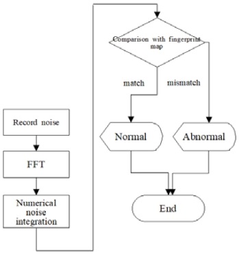
This diagnostic process was categorized into two phases: offline and online. In the offline phase, machine noises that are from normally operating machines are collected in advance, and the noise areas of each noise are calculated. At this time, the noise collection from each machine and the calculation of the noise area are performed repeatedly several times, and their average value is stored into a database as a fingerprint.
Next, in the online phase, the noise from a specific machine is collected in real time and the noise area thereof is calculated. Subsequently, the noise area is compared with the value from the fingerprint map generated in the offline phase (Figure 1).
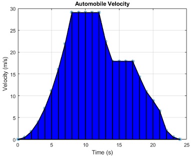
For this, we used a tool that integrated numerically discrete datasets provided by MATLAB. The function code used is trapz(abs(FFT_data)), where FFT_data is the value obtained by the FFT conversion of the input sound source data, and trapz( ) is a function that performs discrete integration by creating a trapezoid using data points [5]. Using this function, the area can be categorized into trapezoidal shapes to calculate the area under the discrete dataset. (Figure 2)
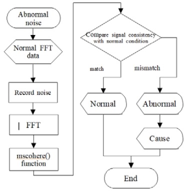
The signal similarity measurement technique can diagnose faults by calculating the consistency between the frequency spectrum of a normal and an abnormal state. This technique uses the mscohere( ) function as a signal comparison analysis tool provided in MATLAB.
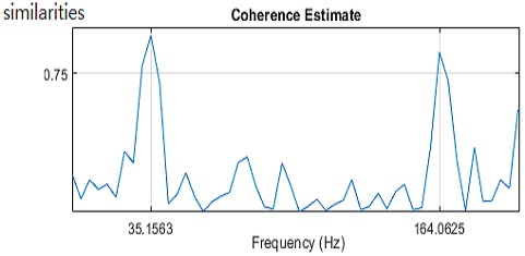
Using the mscohere( ) function, FFT data are transformed to a strength-squared coherence estimation value at a specific frequency to obtain data with a signal similarity between 0 and 1 in all frequency domains as a y-axis value [6]. It can be used to diagnose machine faults as each fault condition has unique noise characteristics. The data representing the inherent noise characteristics can be diagnosed as a fault by estimating the similarity of the normal state data in the same frequency domain. Therefore, if this technique for estimating the similarity between data is used, then the cause of the fault can be analyzed and the fault diagnosed.
Figure 3 shows an example of similarity estimation between two sets of data at a specific frequency domain. Figure 4 depicts the procedure of this technique.
4. Experiments and Performance Evaluation
4.1 Experiment Environment Design
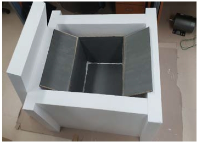
In the noise measurement and analysis experiment, an anechoic chamber was constructed to prevent unnecessary noise from being mixed during machine sound recording.
The anechoic chamber comprised two boxes: a box constructed using styrofoam plates on the outside and a box constructed using paper from the Korea Post box number 6 with a rubber material soundproofing the inside and outside. The paper box was placed inside of the styrofoam box, and then the styrofoam plate was covered and sealed. The anechoic chamber in this experiment was constructed to achieve a double sound insulation effect using the two boxes. (Figure 5).
An electric motor was used as a sample machine in the experiments. Table 1 shows the specifications of the electric motor. A circuit was set to drive the motor and measure the operating sound.
However, when the motor is directly connected to a 220 V power supply in the circuit, it can be extremely dangerous. Therefore, we created a circuit breaker function by connecting the purchased circuit breaker between the power supply and the motor to protect the circuit from an overcurrent. The electric motor was placed in the center of the anechoic chamber, and the chamber was sealed firmly.
After connecting the microphone to the laptop, it was placed in front of the electric motor in the anechoic chamber such that the sound of the operation can be effectively received by the unidirectional microphone. The specifications of the microphone are shown in Table 2.
4.2 Noise Measurement and Analysis
Noise measurement was performed by starting the motor and executing our program in MATLAB. The program received the motor operation sounds from the microphone and recorded them for a certain time period. The motor operation sound was recorded based on the following code [7]:
recorder1 = audiorecorder(48000, 16, 1)
disp('Start');
recordblocking(recorder1, 10);
disp('End');
Furthermore, the motor operation sound was recorded as a WAV formatted file for the next FFT analysis in MATLAB.
The code to generate the operation sound recorded in “recorder1” file as a .wav file is as follows [8]:
filename1 = 'C:\sound.wav';
y1 = getaudiodata(recorder1);
audiowrite(filename1, y1, 48000);
After an FFT conversion of the sound source file obtained from the process above, the code that converted the WAV data into FFT data expressed in the frequency domain is as follows [9]:
N=length(data);
F1=0:fs/N:fs-fs/N;
FFT_data=fft(data);
figure;
plot(F1(1:N), abs(FFT_data(1:N)));
xlabel('Frequency')
ylabel('Amplitude')
grid on
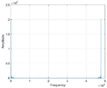
Figure 7 shows a graph of the motor operating sound in the normal state. It is noteworthy that the operating sounds can be analyzed in both the normal and fault states.
When comparing and analyzing the operation sounds, 50 sets of data each for the normal and abnormal conditions were recorded and FFT converted. The average value of the 50 sets of data was calculated to ensure data reliability.
The fault conditions used in the experiments were set to the following conditions:
Foreign substances were mixed in the motor. Front and rear bearings were intentionally damaged. Additionally, other conditions were imposed as the motor casing was not tightened appropriately.
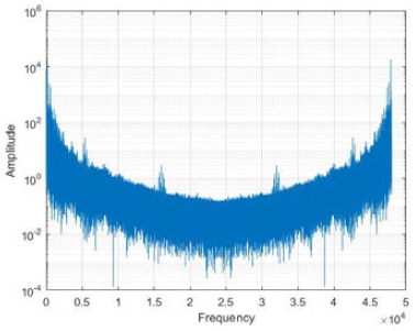
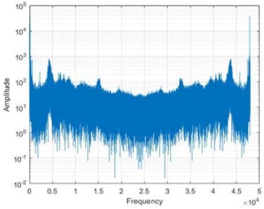
Herein, the average data are shown as frequency–amplitude graphs on y-axis semi-logarithmic scale graphs to improve readability and facilitate analysis.
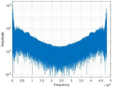
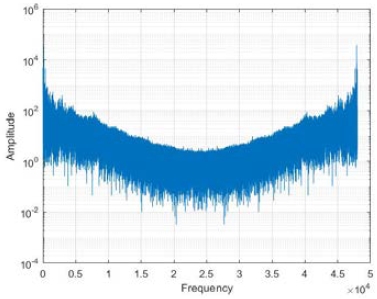
First, the averaged sound in the normal state is shown in Figure 8. As shown, a large amplitude was generated at approximately 30, 120, and 47880 Hz, i.e., at both ends of the entire frequency. In most other frequency domains, no significant amplitude was observed.
Meanwhile, the average sound for the foreign material case exhibited vastly different patterns, as shown in Figure 9. The waveform differed significantly from those at the normal state at 4000, 15000, 33000, 44000 Hz, etc. owing to the friction of the internal foreign material with the rotor. The amplitudes of the sound were larger in the entire frequency spectrum.
Next, the sound generated when two bearings located before and after the shaft in the motor were damaged is shown in Figure 10. The intensity of the amplitude increased significantly compared with that of the normal state at 2000–10000 Hz and 39000–48000 Hz.
Finally, the average sound in the case of vibration and noise due to the casing not being engaged appropriately is shown in Figure 11. High amplitudes in the normal case in the vicinity of 5000, 16000, 32000, and 43000 Hz were not observed. The amplitude values at bands from 2000 to 5000 Hz and 40000 to 47000 Hz were higher than that of the normal state.
The first fault diagnosis technique, i.e., the noise integration technique, was implemented using MATLAB numerical analysis tools based on the characteristics of the frequency and amplitude of each state devised above, as well as the average value from the FFTed sounds.
4.3 Results of Diagnostic Techniques
Based on the experimental results above, the noise integration technique was applied. In the offline phase of the technique, a fingerprint map (normal noise area) was created. In the online phase, the noise area of each fault state was obtained. Table 3 shows the results of the fault diagnosis technique.
The area value in Table 3 is the value obtained by integrating the average value after recording and averaging 50 times for each condition under the same measurement conditions.
The noise area value was derived as follows:
- 1. The operating sound of the motor for each condition was recorded and saved as sound source data. (data1~50)
- 2. The saved sound source files were loaded as data in MATLAB, FFT was performed, and the average value was calculated. (FFT1~50, FFT_mean)
- 3. By applying the absolute average value of the obtained FFT data to the trapz function, the noise area value for each condition was derived. (Noise area=trapz(abs(FFT_data)))
By performing this process, the reliability of the diagnosis reference fingerprint map can be increased.
The normal noise area differs significantly from other noise areas. If these differences are outside the range of the normal state, then they can be diagnosed an abnormal.
However, the external background noise during diagnosis in the actual field is a non-negligible factor when using this technique; therefore, we performed an additional experiment.
The mixed noise resulting from the diesel engine noise and motor noise without a tightened casing occurring simultaneously was recorded. For comparing, the diesel engine noise and loosed motor noise were recorded separately. The noise areas of the three noises were obtained using our program. The results are shown in Table 4.
The noise area value of the engine noise was extracted from the noise area of the mixed noises, i.e., 1.4738 × 10⁷ (= 6.2768 × 10⁷ - 4.8030 × 10⁷). Comparing this area value with the engine noise recorded separately (1.6707 × 10⁷), it was confirmed that an excellent match was obtained even though the engine noise source from the speaker was used owing to the limitations of the experimental environment.
However, in actual environments, the difference value can be calculated using the average data accumulated from mixed noises, background noise, and device noise. When utilizing these real noise data, faults can be diagnosed even when the noises of the field are mixed.
In the initial study pertaining to the signal similarity measurement technique, data analysis was not well performed because the signal similarity calculation results were inconsistent. Therefore, as a result of careful analysis, it was discovered that the cause was the recording sound.
The mscohere( ) function, which measures the similarity of FFT data of two operating sounds, calculates the y-value of signal similarity between 0 and 1 for each frequency x-value. When viewing the frequency spectrum of the sound recorded in the early study with the naked eye, the spectra under the same conditions almost matched with each other. Therefore, a simple similarity measurement was expected to enable diagnosis; however, this was not achieved.
This problem is explained as follows: When the average value of the normal state FFT data and the data of 50 foreign matter mixing conditions are measured for signal similarity, if the normal state average value and the foreign substance mixing condition are 60% identical, then all 50 similarities should be approximately 0.6; however, in the actual results, the consistency values indicated a large deviation.
In other words, because the operating sound of the electric motor was not constant because it was generated by the rotation of the rotor, the arrangement of the frequency value and amplitude between the two sound sources was not always the same and a certain difference would be indicated even if the same sound was heard.
Therefore, if the amplitude difference for each frequency of each sound source is not resolved, then it will be difficult to diagnose a fault. Therefore, a method to reduce this error and output a consistent similarity value was investigated.
Consequently, a frequency interval mean technique was devised. If the arrangement of amplitude values for each frequency for each sound source is not the same and the signal similarity is difficult to compare accurately owing to the large amount of data, the problem will be solved based on the hypothesis that the error can be reduced by averaging each interval after segmenting the entire frequency section. This method has been demonstrated successful in previous studies.
When the experiment was conducted by applying this improvement method, a consistent similarity was derived for each condition, unlike the previous similarity values with large deviations, and the average value of the similarities indicated a clear difference in distinguishing the cause of failure for each condition. The details of the experiment are as follows.
For the analysis of each condition, first, the average value of the FFT data in the steady state was calculated with the similarity of 50 normal state data to obtain a reference value that can be determined to be a steady state; subsequently, it was compared with the value from the existing similarity measurement to determine the improvement gained.
First, the frequency x-values of 480,000 data from the normal-state FFT average value were segmented into 480 groups by 1000 and averaged for each group.
Subsequently, by measuring the signal similarity with each of the 50 sets of data in the normal state, the performance difference obtained by using and not using the frequency averaging technique can be confirmed.
The MATLAB code used in the process is as follows:
FFT=fft(data);
A=reshape(FFT,1000,480);
FFT_m=mean(A);
mean(mscohere(FFT_avg, FFT_m));
mscohere(FFT_avg, FFT_m);
If the mscohere( ) function is input, then the similarity graph for each frequency can be output; if it is input to the mean function, the average of the similarity for each frequency can be obtained.
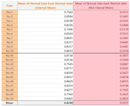
Hence, when the interval mean technique was applied and the average of 50 similarity measurements was obtained, a high agreement rate of 0.8248 was indicated; meanwhile, when it was not applied, a low agreement rate of 0.5031 was indicated, and a large deviation was observed for each agreement value. A comparison of the results is shown in tabular form in Figure 12.
The technique of reducing the deviation of the signal similarity by segmenting the frequency x-value into 1000 units and averaging it improved the signal similarity by approximately 39%.
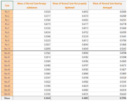
Therefore, based on the improvement method above, the results of measuring the similarity between the normal state and the signal for each failure condition are as shown in the table in Figure 13.
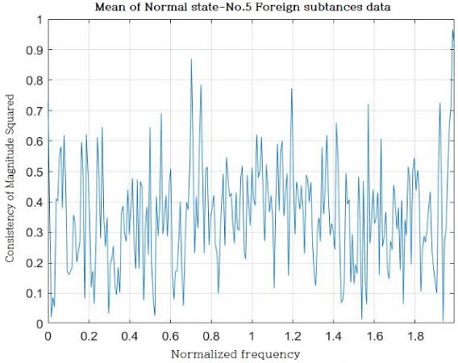
In addition, a graph that measures the degree of similarity is presented based on the state of foreign matter mixing as an example such that it can be confirmed using a visual indicator. (Figure 14).
The table of measurement results shows that the similarity decreased significantly when a failure occurred compared with the signal similarity value in the normal state.
In addition, it was confirmed that the degree of similarity for each failure condition differed significantly. If the signal similarity measurement technique is applied, then the cause of failure can be determined during failure diagnosis.
Hence, it was confirmed that the signal similarity measurement technique yielded a higher diagnostic accuracy and a better fault cause determination function than the numerical data integration technique.
5. Conclusion
Herein, two fault diagnosis techniques were proposed to effectively diagnose motor faults that were undetectable by the AMS. Two techniques were implemented in this study: the noise integration technique and the signal similarity measurement technique, as a program in MATLAB. Based on the frequency spectrum obtained experimentally, the steady normal and fault states indicated significant differences visually and numerically.
Hence, more objective and precise comparisons were enabled by recording and averaging the values obtained from the 50 trials of experiments for each condition under the same measurement environment. In addition, it was possible to visualize and quantify sound wave data through the program. In previous studies, the frequency spectrum had to be directly compared based on the noise characteristics for each condition and diagnosed as whether it contained faults.
However, in this study, fault diagnosis was enabled by integrating the values of digitized FFT data. Because only one value, i.e., the noise area value, was used for diagnosis, the diagnosis time was reduced significantly.
In the signal similarity measurement technique, a problem occurred in data processing during the research process; however, it can be overcome by applying the data section integration technique. The signal similarity measurement technique demonstrated a higher diagnostic accuracy than the conventional noise integration technique; additionally, it can analyze the cause of failure using the result value.
In conclusion, in diagnosing motor failure, the noise integration technique can perform diagnosis rapidly when simply determining a normal or malfunction state. Meanwhile, the signal similarity measurement technique requires a longer time, but it can accurately analyze the motor condition and the cause of failure.
Author Contributions
Conceptualization, J. Kang and Y. Oh; Methodology, J. Kang, Y. Oh, and H. Im; Software, J. Kang and Y. Oh; Formal Analysis, H. Im and M. Park; Investigation, D. Kim, M. Park, and H. Im; Resources, J. Son and H. Im; Data curation J. Kang; Writing-Original Draft Preparation, J. Son and J. Kang; Writing-Review & Editing, J. Son, J. Kang, and D. Kim; Visualization, J. Son and J. Kang; Supervision, J. Son; Project Administration, J. Son; Funding Acquisition, J. Son.
References
-
I. Tawiah, et al., “Marine engine room alarm monitoring system,” International Journal of Advanced Computer Science and Applications, vol. 9, no. 6, pp. 433-441, 2018.
[https://doi.org/10.14569/IJACSA.2018.090659]

- S. -J. Park, “Fault Diagnosis of a Pump Using Analysis of Noise,” M. S. Thesis, Department of Mechanical Engineering, Kunsan University, Korea, 2004 (in Korean).
- Y. -C. Na, N. H. Byun, J. S. Lee, G. S. Kim, and S. K. Hong, “A study on motor fault analysis using the vibration and the noise, 2014 fall conference of the Korean Institute of Electrical Engineers, pp. 78-79, 2014 (in Korean).
- D. -J. Choi, J. H. Han, S. W. Park, and S. K. Hong, “Comparison of characteristics of noise and vibration data for diagnosis of deep learning motor fault,” 2019 Spring conference of the Korean Institute of Electrical Engineers, pp. 46-47, 2019 (in Korean).
- MATLAB, Integration of Numeric Data, https://kr.mathworks.com/help/matlab/math/integration-of-numeric-data.html, , Accessed July 19, 2020.
- MATLAB, Measuring-Signal-Similarities, https://kr.mathworks.com/help/signal/examples/measuring-signal-similarities.html, , Accessed August 18, 2020.
- MATLAB, Audio Record and Play, https://kr.mathworks.com/help/matlab/import_export/record-and-play-audio.html, , Accessed June 10, 2020.
- MATLAB, Audio Write, https://kr.mathworks.com/help/matlab/ref/audiowrite.html, , Accessed June 10, 2020.
- MATLAB, Fast Fourier Transform (FFT), https://kr.mathworks.com/help/matlab/ref/fft.html, , Accessed June 15, 2020.

