The Korean Society of Marine Engineering

[ Original Paper ]

Journal of Advanced Marine Engineering and Technology - Vol. 44, No. 1, pp.42-47

ISSN: 2234-7925 (Print) 2234-8352 (Online)

Print publication date 29 Feb 2020

Received 19 Jul 2019 Revised 20 Nov 2019 Accepted 13 Dec 2019

DOI: https://doi.org/10.5916/jamet.2020.44.1.42

Sensorless speed control of a permanent magnet synchronous motor using an unscented Kalman filter with compensated covariances

Cheol Moon¹ ; Young-Ahn Kwon^†

1Doctoral Researcher, School of Electrical and Computer Engineering, Pusan National University, Tel: 051-510-3086 chmoon@pusan.ac.kr

Correspondence to: ^†Professor, School of Electrical and Computer Engineering, Pusan National University, 2, Busandaehak-ro 63 beon-gil, Geumjeong-gu, Busan, 46241, Korea, E-mail: yakwon@pusan.ac.kr, Tel: 051-510-2372

Copyright ⓒ The Korean Society of Marine Engineering
This is an Open Access article distributed under the terms of the Creative Commons Attribution Non-Commercial License (http://creativecommons.org/licenses/by-nc/3.0), which permits unrestricted non-commercial use, distribution, and reproduction in any medium, provided the original work is properly cited.

Abstract

This study investigates the unscented Kalman filter with compensated covariances for the sensorless speed control of a permanent magnet synchronous motor. The unscented Kalman filter features a direct transformation process involving unscented transformation for removing the linearization process error that may occur in the extended Kalman filter. However, the Kalman filter should consider the covariance values for the system and measurement noises, and it is challenging to compute appropriate covariance values for the system and measurement noises in the design process. The covariance values are usually obtained from experience or by the trial-and-error method in the sensorless speed control of a permanent magnet synchronous motor. However, this process may be incorrect. This paper proposes an unscented Kalman filter with a fuzzy tuner for compensating covariance values in the sensorless speed control of a permanent magnet synchronous motor.

Keywords:

Unscented Kalman filter, Covariance compensation, Permanent magnet synchronous motor, Sensorless control

1. Introduction

The vector control of a permanent magnet synchronous motor allows for high-performance operation and control, and it is widely used in many fields, including industrial uses. Speed and position information are required to perform vector control of a permanent magnet synchronous motor. However, position detectors require additional space for installation and adds to the cost of the motor. Moreover, the detector’s reliability may be reduced by the surrounding operating environment. Therefore, researchers are studying several sensorless algorithms that allow for speed and position detectors to be omitted [1]-[4]. Among these sensorless algorithms, a method that uses an extended Kalman filter is known for being robust against noise [5]-[9]. The extended Kalman filter observer estimates state variables through a Kalman gain and recursive state values. However, compared to other methods, the extended Kalman filter uses a complex algorithm, and it ignores higher-order terms in the linearization process that uses a Jacobian matrix. As such, a margin of error occurs between its estimates and actual systems. An unscented Kalman filter overcomes this linearization problem by using an unscented transformation rather than a linearization process. As such, it shows a marked difference from the extended Kalman filter, and it is currently the subject of a great deal of research [10]-[15]. The covariance matrix values for the systems and noise that are considered by the Kalman filter are described as Gaussian white noise. In most cases, these values are found through experience or trial and error, which is challenging. This paper proposes and verifies the validity of a new sensor-less speed control method for permanent magnet synchronous motors that use an unscented Kalman filter, which compensates the covariance using fuzzy tuners.

2. Mathematical Model of Permanent Magnet Synchronous Motor

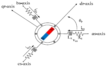
The permanent magnet synchronous motor used in this study is cylinder-shaped. Figure 1 shows an equivalent model of the permanent magnet synchronous motor [1][2].

Figure 1:

The equivalent model of the permanent magnet synchronous motor

The permanent magnet synchronous motor’s real-axis stator voltage equation is as follows.

v a s v b s v c s = R s 00 0 R s 0 00 R s i a s i b s i c s + d s t λ a s λ b s λ c s

(1)

v_xs, i_xs, and λ_xs are stator phase voltages, current, and linkage magnetic flux, respectively. R_s is the stator winding’s equivalent resistance.

The linkage magnetic flux of each stator phase is as follows.

λ a s λ b s λ c s = L s 00 0 L s 0 00 L s i a s i b s i c s + K e cos ⁡ θ r cos ⁡ θ r - 23 π cos ⁡ θ r - 43 π

(2)

L_s is the stator inductance, K_e is the back emf constant, θ_r is the electrical rotor angle.

The back electromotive force of each stator phase from Equation (1) and Equation (2) is as follows.

e a s e b s e c s = - w r K e sin ⁡ θ r sin ⁡ θ r - 23 π sin ⁡ θ r - 43 π

(3)

w_r is the electrical rotor speed.

Coordinate transformation is performed for vector control of a permanent magnet synchronous motor. If the coordinates are transformed into a stationary reference frame that is based on the stator axis and a synchronous reference frame that is based on the rotor axis, Equation (1) and Equation (3) become the equations shown below, respectively.

v α s v β s = R s + d d t L s 0 0 R s + d d t L s i α s i β s + e α s e β s

(4)

e α s e β s = w r K e - sin ⁡ θ r cos ⁡ θ r

(5)

v d r v q r = R s + L s d d t - w r - w r R s + L s d d t i d r i q r + e d r e q r

(6)

e d r e q r = w r K e - 1 1

(7)

If the number of poles in the permanent magnet synchronous motor is P, the torque values that occur in the stationary reference frame and the synchronous reference frame are as shown below, respectively.

T e = P 2 32 K e - sin ⁡ θ r i α s + cos ⁡ θ r i β s

(8)

T e = P 2 32 K e i q r

(9)

The mechanical equation of a PMSM is as follows.

T e = J m d w m d t + B m w m + T L

(10)

J_m is the inertia coefficient, B_m is the friction coefficient, W_m is the mechanical speed of the rotor, and T_L is the load torque.

Below is the state equation for the permanent magnet synchronous motor that uses the current and back electromotive force in the stationary reference frame from Equation (4) and Equation (5) as state variables.

x ˙ = Ax + Bu

(11)

y = Cx

(12)

x = i α s i β s e α s e β s T, u = v α s v β s T,

y = i α s i β s T

A = A 11 A 12 A 21 A 22, B = B 11 B 21, C = C 11 C 12

A 11 = - R s L s I, A 12 = - 1 L s I, A 21 = 0, A 22 = w r 0 - 1 10,

B 11 = 1 L s I, B 21 = 0, C 11 = I, C 12 = 0 .

The discrete-time nonlinear state equations including the system and measurement noises in a PMSM drive are as follows.

x k + 1 = f x k, u k + w k

(13)

y k = h x k + v k

(14)

w_k is the system noise, and v_k is the measurement noise.

3. Unscented Kalman Filter

The unscented Kalman filter has the advantage of using an unscented transformation to omit the linearization process that is performed by the extended Kalman filter. The extended Kalman filter ignores higher-order terms in the linearization process, which uses a Jacobian matrix. As such, a margin of error occurs between its estimates and actual systems. The unscented transformation in the unscented Kalman filter performs estimations by using sigma points and weights to create suitable samples according to the number of state variables. By deciding upon the sigma points and weights, the unscented Kalman filter can perform accurate estimations with a smaller number of samples than other stochastic estimation methods. In the unscented transformation, the sigma points and weight values can vary according to the scaling parameters, and there are several types of methods, such as the basic unscented transformation and the general unscented transformation [16][17]. The unscented transformation’s accuracy is generally proportional to the number of samples. However, an increase in the number of samples causes an increase in the computation time. The sigma point is found through the error covariance, and the weight is a constant that determines the importance of the estimated values. The scaling parameter determines each estimate value assignment. The unscented transformation’s sigma points and weights are calculated as shown below by finding the upper triangle matrix from the error covariance using Cholesky decomposition.

U T U = n + k P x

(15)

x 0 = x^, x i = x^+ u i, x i = n = x^- u i

(16)

W 0 = k n + k, W i = 1 2 n + k, W i + n = 1 2 n + k

(17)

P_x is the error covariance matrix, and n is the dimension of the state variable matrix. u_i is a row vector of U. i = 1, 2, ⋯ , n.

In the basic unscented transformation, the scaling parameter value is 0, and the 0th sigma point and weight are removed. Therefore, the number of sigma points in the basic unscented transformation is 2n². Each weight has a fixed value of 1/2n. In the general unscented transformation, the number of sigma points is 2n² + n. As the number of sigma points increases, the relative accuracy of the unscented transformation, and the computation time also increase.

The unscented Kalman filter, which uses an unscented transformation to omit the linearization process, can generally be divided into the stages of sigma point and weight calculation, prediction, Kalman gain calculation, and estimation. It consists of the process below [10][11].

1) Initialization
2) Calculation of sigma points and weights
3) Relative variable value estimation and error covariance calculation

x^k ¯ = ∑ i = 0 2 n W i f x i

(18)

P x ¯ = ∑ i = 0 2 n W i f x i - x^k ¯ f x i - x^k ¯ T + Q

(19)

4) Output variable value estimation and error covariance calculation

y^k ¯ = ∑ i = 0 2 n W i h x i

(20)

P y = ∑ i = 0 2 n W i h x i - y k^h x i - y^k T + R

(21)

5) Kalman gain calculation

P x y = ∑ i = 0 2 n W i f x i - x^k ¯ h x i - y^k ¯ T

(22)

K k = P x y P y - 1

(23)

6) State variable and error covariance updating

x^k = x^k ¯ + K k y k - y^k

(24)

P x = P x ¯ - K k P y K k T

(25)

Here, the matrices Q and R are covariance matrices for the system noise and measurement noise, respectively. The System noise and measurement noise have an average of 0, and they are Gaussian noise with a standard distribution. In the covariance matrices Q and R, there is no correlation between the noise. Therefore, they are each diagonal matrices.

4. Fuzzy Tuner for Compensated Covariance

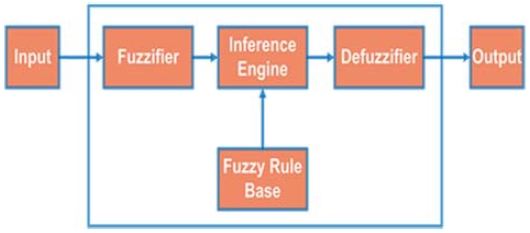
Generally, the covariance matrices Q and R are found through experience or trial and error; however, it is challenging to find accurate values [18]-[21]. This paper proposes a new sensor-less speed control method for a permanent magnet synchronous motor that uses an unscented Kalman filter that compensates for covariance using a fuzzy tuner. Generally, fuzzy systems consist of three parts, as shown in Figure 2 [22]-[25]. The first step is the fuzzification step that converts the input data set into a fuzzy set using fuzzy linguistic variables or a membership function. In the second step, the inference system creates a rule base in which the fuzzified membership function is mapped to the output membership function set. The last step is defuzzification, in which the output membership function is transformed into actual output values.

Figure 2:

The conventional fuzzy system

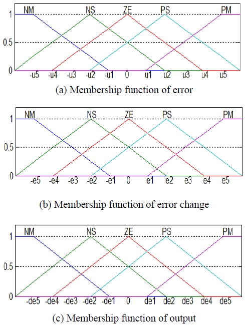
Fuzzy inferences in this study used the Mandani inference method. Table 1 shows the fuzzy rule base and Figure 3 shows the membership function of the fuzzy variables. The output for the input used the maximum-minimum synthesis rule. Defuzzing was performed using the geometric center method. Fuzzy rule base errors are output errors from the permanent magnet synchronous motor sensor-less drive system, i.e., margins of error between the estimated current and the measured current. The fuzzy tuner output determined new covariance values.

Table 1:

The fuzzy rule-base

Figure 3:

Membership function of the fuzzy variables

5. Simulation and Discussions

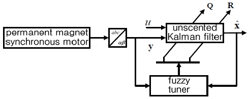
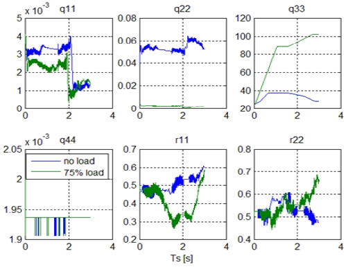
Simulations were performed to verify the validity of the proposed unscented Kalman filter method that compensates the covariance using a fuzzy tuner as a sensorless speed control method for permanent magnet synchronous motors. The permanent magnet synchronous motor’s rated power, voltage, current, and speed were 1 hp, 200 V, 5.4 A, and 2000 rpm, respectively. Figure 4 is a block diagram of the proposed unscented Kalman filter method that compensates the covariance. Matrices Q and R are the covariance matrices for the system noise and measurement noise, respectively. They are diagonal matrices with no correlation between the noises. Q = diag[q₁₁ q₂₂ q₃₃ q₄₄], and R = diag[r₁₁ r₂₂].

Figure 4:

Block diagram of the UKF with compensated covariance

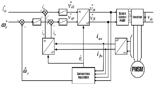
Figure 5 shows a block diagram of the proposed permanent magnet synchronous motor’s overall sensorless drive system.

Figure 5:

Configuration of overall system

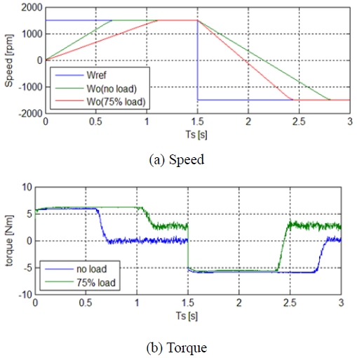
Figure 6 and Figure 7 show the results of running the aforementioned permanent magnet synchronous motor sensorless drive system at no load and at a 75 % rated load. The speed and torque responses and the changes in the covariance values are shown. As shown in the results, the changes in the covariance values caused by the fuzzy tuner are beneficial for the speed and torque responses.

Figure 6:

The speed and torque responses

Figure 7:

The variation of the covariance values

6. Conclusions

The extended Kalman filter, which is a method of sensorless speed control for permanent magnet synchronous motors, is known to be robust against system and measurement noise. However, a margin of error can occur between its estimates and actual systems during the process of linearizing nonlinear systems, and this can lead to system instability. The permanent magnet synchronous motor sensorless speed control method that uses an unscented Kalman filter has the advantage of omitting the linearization process by performing an unscented transformation. Furthermore, the covariance matrix values that are set in a Kalman filter are typically found through experience or trial and error, but it is challenging to obtain accurate values. This paper proposes an unscented Kalman filter method that compensates the covariance using a fuzzy tuner as a new sensorless speed control method for permanent magnet synchronous motors. As shown in the results, the covariance compensation was properly performed in various conditions, such as no-load, load, and variable speed.

Acknowledgments

This work was supported by a 2-Year Research Grant of Pusan National University.

Author Contributions

Conceptualization, C. Moon and Y. A. Kwon; Methodology, C. Moon; Software, C. Moon; Validation, C. Moon and Y. A. Kwon; Writing—Original Draft Preparation, C. Moon; Writing—Review & Editing, Y. A. Kwon; Visualization, C. Moon; Supervision, Y. A. Kwon; Project Administration, Y. A. Kwon.

References

K. Rajashekara, A. Kawamura, and K. Matsuse, Sensorless Control of AC Motor Drives, IEEE Press, 1996.
J. Holtz, “State of the art of controlled AC drives without speed sensors,” International Journal of Electronics, vol. 80, no.2, pp. 249-263, 1996. [https://doi.org/10.1080/002072196137444]
I. Boldea, “Control issues in adjustable speed drives,” IEEE Transactions on Energy Conversion, vol. 33, no. 4, pp. 32-50, 2008. [https://doi.org/10.1109/MIE.2008.928605]
C. Liu, K. T. Chau, L. Kirtley, C. C. Chan, K. Rajashekara et al, “Guest editorial emerging electric machines and drives for smart energy conversion,” IEEE Transactions on Energy Conversion, vol. 33, no. 4, pp. 1931-1933, 2018. [https://doi.org/10.1109/TEC.2018.2879231]
R. Dhaouadi, N. Mohan, and L. Norum, “Design and implementation of an extended kalman filter for the state estimation of a permanent magnet synchronous motor,” IEEE Transactions on Power Electronics, vol. 6, no. 3, pp. 491-497, 1991. [https://doi.org/10.1109/63.85891]
Z. Zedong, L. Yongdong, M. Fadel, X. Xi, “A rotor speed and load torque observer for PMSM based on extended kalman filter,” IEEE International Conference of Industrial Technology, pp. 233-238, 2006. [https://doi.org/10.1109/ICIT.2006.372295]
Z. Xu and M. F. Rahman, “Comparison of a sliding observer and a kalman filter for direct-torque-controlled IPM synchronous motor drives,” IEEE Transactions on Industrial Electronics, vol. 59, no. 11, pp. 4179–4188, 2012. [https://doi.org/10.1109/TIE.2012.2188252]
F. Alonge, T. Cangemi, F. D'Ippolito, A. Fagiolini, and A. Sferlazza, “Convergence analysis of extended kalman filter for sensorless control of induction motor,” IEEE Transactions on Industrial Electronics, vol. 62, no. 4, pp. 2341-2352, 2015. [https://doi.org/10.1109/TIE.2014.2355133]
E. Zerdali, “Adaptive extended kalman filter for speed-sensorless control of induction motors,” IEEE Transactions on Energy Conversion, vol. 34, no. 2, pp. 789-800, 2019. [https://doi.org/10.1109/TEC.2018.2866383]
S. J. Julier, J. K. Uhlmann, and H. F. Durrant-Whyte, “A new approach for filtering nonlinear systems,” Proceedings of American Control Conference, vol.3, pp.1628 – 1632, 1995.
S. Julier, J. Uhlmann, and H. F. Durrant-Whyte, “A new method for the nonlinear transformation of means and covariances in filters and estimators,” IEEE Transactions on Automatic Control, vol. 45, no. 3, pp. 477–482, 2000. [https://doi.org/10.1109/9.847726]
T. F. Chan, P. Borsje, and W. Wang, “Application of unscented kalman filter to sensorless permanent-magnet synchronous motor drive,” IEEE International Electric Machines and Drives Conference, pp. 631–638, 2009. [https://doi.org/10.1109/IEMDC.2009.5075272]
D. Janiszewski, “Load torque estimation in sensorless PMSM drive using unscented kalman filter,” IEEE International Symposium on Industrial Electronics, pp. 643–648, 2011. [https://doi.org/10.1109/ISIE.2011.5984233]
C. Moon and Y. A. Kwon, “Sensorless speed control of permanent magnet synchronous motor by unscented kalman filter using various scaling parameters,” Journal of Electrical Engineering & Technology, vol. 11, no. 2, pp. 347-352, 2016. [https://doi.org/10.5370/JEET.2016.11.2.347]
H. Zhou, Z. Liu, and X. Yang, “Motor torque fault diagnosis for four wheel independent motor-drive vehicle based on unscented kalman filter,” IEEE Transactions on Vehicular Technology, vol. 67, no. 3, pp. 1969-1976, 2018. [https://doi.org/10.1109/TVT.2017.2751750]
S. J. Julier, “The scaled unscented transformation,” Proceedings of American Control Conference, vol. 6, pp. 4555-4559, 2002. [https://doi.org/10.1109/ACC.2002.1025369]
S. J. Julier, “The spherical simplex unscented transformation,” Proceedings of American Control Conference, vol. 3, pp. 2430-2434, 2003.
S. Bolognani, L. Tubiana, and M. Zigliotto, “Extended kalman filter tuning in sensorless PMSM drives,” IEEE Transactions on Industrial Applications, vol. 39, no. 6, pp. 1741–1747, 2003. [https://doi.org/10.1109/TIA.2003.818991]
N. Salvatore, A. Caponio, F. Neri, S. Stasi, and G. L. Cascella, “Optimization of delayed-state kalman-filterbased algorithm via differential evolution for sensorless control of induction motors,” IEEE Transactions on Industrial Electronics, vol. 57, no. 1, pp. 385-394, 2010. [https://doi.org/10.1109/TIE.2009.2033489]
M. Saha, R. Ghosh, and B. Goswami, “Robustness and sensitivity metrics for tuning the extended kalman filter,” IEEE Transactions on Instrumentation and Measurement, vol. 63, no. 4, pp. 964-971, 2014. [https://doi.org/10.1109/TIM.2013.2283151]
M. Ahmeid, M. Armstrong, S. Gadoue, M. Al-Greer, and P. Missailidis, “Real-time parameter estimation of DC– DC converters using a self-tuned kalman filter,” IEEE Transactions on Power Electronics, vol. 32, no. 7, pp. 5666-5674, 2017. [https://doi.org/10.1109/TPEL.2016.2606417]
D. Driankov, H. Hellendoorn, and M. Reinfrank, An Introduction to Fuzzy Control, Springer Science & Business Media, 2013.
J. M. Mendel, “Fuzzy logic systems for engineering: A tutorial,” Proceedings of the IEEE, vol. 83, no. 3, pp. 345-377, 1995. [https://doi.org/10.1109/5.364485]
S. Bayhan, S. Demirbas, and H. Abu-Rub, “Fuzzy-PI-based sensorless frequency and voltage controller for doubly fed induction generator connected to a DC microgrid,” IET Renewable Power Generation, vol. 10, no. 8, pp. 1069-1077, 2016. [https://doi.org/10.1049/iet-rpg.2015.0504]
J. Yang, B. Huang, H. Shen, D. Xie, F. Xiong, S. Lu, and H. Chen, “EKF based fuzzy PI controlled speed sensorless power optimal control of a direct drive power system,” IEEE Access, vol. 7, pp. 61610-61619, 2019. [https://doi.org/10.1109/ACCESS.2019.2912431]

		⊿e
		NM	NS	ZE	PS	PM
e	NM	NM	NM	NM	NS	ZE
	NS	NM	NM	NS	ZE	PS
	ZE	NM	NS	ZE	PS	PM
	PS	NS	ZE	PS	PM	PM
	PM	ZE	PS	PM	PM	PM

		⊿e
		NM	NS	ZE	PS	PM
e	NM	NM	NM	NM	NS	ZE
	NS	NM	NM	NS	ZE	PS
	ZE	NM	NS	ZE	PS	PM
	PS	NS	ZE	PS	PM	PM
	PM	ZE	PS	PM	PM	PM

		⊿e
		NM	NS	ZE	PS	PM
e	NM	NM	NM	NM	NS	ZE
	NS	NM	NM	NS	ZE	PS
	ZE	NM	NS	ZE	PS	PM
	PS	NS	ZE	PS	PM	PM
	PM	ZE	PS	PM	PM	PM

		⊿e
		NM	NS	ZE	PS	PM
e	NM	NM	NM	NM	NS	ZE
	NS	NM	NM	NS	ZE	PS
	ZE	NM	NS	ZE	PS	PM
	PS	NS	ZE	PS	PM	PM
	PM	ZE	PS	PM	PM	PM