Level control of single water tank systems using Fuzzy-PID technique
In this study, for the control of a single water tank system, a fuzzy-PID controller design technique based on a fuzzy model is investigated. For this purpose, a water tank system is linearized as a number of submodels depending on the operating point, and a fuzzy model is obtained by fuzzy combining. Each submodel is approximated as a first order time delay model, and a PID controller is designed using several existing tuning techniques. Then, through the fuzzy combination of this controller using the same method as that of the fuzzy model, a fuzzy-PID controller is designed. For the proposed technique, a simulation is performed using the fuzzy model of a water tank system, and the validity is examined by comparing its performance with that of a PID controller.
Keywords:
Single tank level control system, Fuzzy model, First order time delay model, PID controller, fuzzy PID controller1. Introduction
Recently, the most common control problem for the process of an industrial site is to control various variables such as the temperature, water level, and internal pressure of a tank and a chemical reactor [1]. Especially, for the process such as oil and chemical liquid, the most important element is to control the liquid level of a tank. The purpose of level control is to make the water level follow a given set value or to quickly restore a constant water level in case of disturbance. In general, a PID controller is widely used for level control; and the gains of the controller should be tuned so that the required performance of a controlled system can be satisfied. This tuned PID controller can satisfy the required performance of the controlled system when the operating environment of the controlled system is unchanged. However, if the parameters of the controlled system change due to the change in the operating environment of the controlled system, satisfactory control cannot be guaranteed unless the gains of the controller are artificially changed again.
For a level control system the parameters of the system change significantly depending on the operating point as mentioned above, and thus, the required control performance cannot be guaranteed using one controller. However, in most studies on level control [2]-[5], a linear model was obtained from one operating point, and then, a controller was designed at the operating point.
Therefore, in this study, to resolve this problem, a following two-stage design process is proposed. First, submodels that model the water level of a tank (i.e., controlled system) by dividing it into several sections are considered. In this regard, the time constant and gain of each submodel are obtained through an experiment. A fuzzy model that is made by the fuzzy combination of the submodels obtained through the above process is regarded as the non-linear model of the water tank system. Then, to control each submodel, a sub-PID controller is designed. Through the fuzzy combination of the sub-PID controller, a fuzzy-PID controller that enables flexible and appropriate level control even when the water level changes is designed.
The validity of the proposed method is verified based on a simulation through the application to the non-linear fuzzy model of the level control system.
2. Level Control System
For the modeling of a level control system, a single water tank system shown in Figure 1 is considered.

Single water tank system
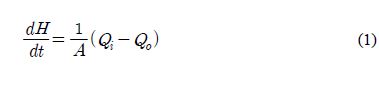
Qi[㎤/s], Qo [㎤/s], H [cm], and A [cm2] represent the inflow rate of the water tank, the outflow rate, the water level, and the cross sectional area of the tank, respectively.
If the inflow rate of the water tank, Qi, and the outflow rate of the tank outlet, Qo , are equal, the water level of the water tank, H, maintains a constant equilibrium state. In this regard, the water tank system can be modeled as a single-input single-output (SISO) system regarding the relation between the input, Qi, and the output, H.
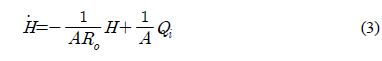
For the water level in an equilibrium state shown in Figure 1, the water level changes when the inflow rate or the outflow rate changes, and the rate of level change can be expressed as follows.
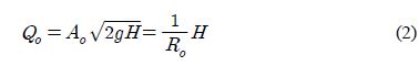
Based on Bernoulli’s equation, the speed at the water tank outlet is expressed as
 [㎝/s]; and a flow rate [㎤/s] can be obtained when this speed is multiplied by the cross sectional area of the water tank outlet, Ao [cm2]. Therefore, the outlet flow rate, Qo , can be expressed as follows, and also can be expressed using the fluid resistance at the water tank outlet, Ro .
Based on Equations (1) and (2), the relation between the inflow of the water tank and the water level can be expressed as follows.
The flow control valve, which determines the inflow of the water tank, generally has a high reduction gear ratio of the power transmission elements, and a high frictional resistance of the valve part. Thus, it can be regarded as a first order linear model as shown in Equation (4).
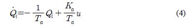
where u[v] is the input voltage of the control valve, Kα[㎤/(s·V)] is the gain of the control valve, and Tα[s] is the time constant of the control valve.
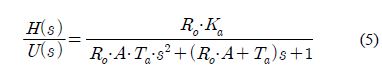
For the block diagram of the water tank system (i.e., controlled system), the transfer function of the output, H(s), for the input, U(s), can be obtained as shown in Equation (5).
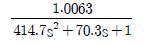
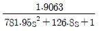
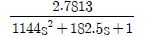
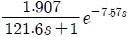
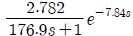
In this study, the water tank was modeled as summarized in Table 1 through an experiment when the steady state water level was 4[cm], 8[cm], and 12[cm], respectively. These three models are defined as submodels, and are expressed as sub-MDi (i=1, 2, and 3).

The transfer functions of tank system
3. Design of the controller
2.1 PID controller
A standard PID controller is implemented by the parallel combination of proportional action, integral action, and derivative action; and is expressed using a transfer function as shown in Equation (6).
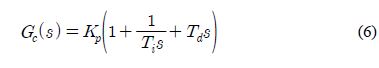
where KpTd and Td represent the proportional gain, the integral time, and the derivative time, respectively. Proportional action reduces the rise time by amplifying the current error, but a steady state error exists when the controlled system is “0” type. Integrative action can eliminate a steady state error by amplifying the cumulative error from the past to the present, but transient response could deteriorate if the gain is wrongly adjusted. Derivative action amplifies the rate of change of an error. Thus, if derivative action is added to a PI-type controller and is properly used, overshoot can be decreased, and transient response can be improved. Therefore, the design of a desirable PID controller comes down to the problem of adjusting the parameters of the controller so that the output can follow the change in the set value.
Figure 2 shows the control system, where the controlled system and the PID controller have been combined. The error, E(s), can be expressed using the set value, R(s), and the disturbance, D(s), as shown in Equation (7).
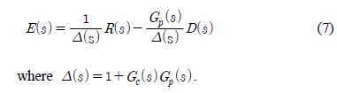

Unit feedback PID control system
As mentioned earlier, a PID controller is widely used to improve set value following performance or disturbance suppression performance. The existing tuning methods of a PID controller include the Z-N method [6], the C-C method [7], the IMC method [8], and the Lopez method [9]. On the other hand, Kim et al. [10] proposed a model-based tuning rule using RCGA, and showed that its performance is superior to that of the existing method.
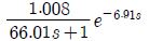
The tuning method mentioned above requires a process in which a high order controlled system is approximated as a first order plus time delay(FOPTD) model. In this study, the submodels are approximated as FOPTD models using least square method (LSM), and the estimated models are summarized in Table 2.
The FOPTD models obtained from LSE
For each FOPTD model, a sub-PID controller can be designed using the existing tuning methods, as summarized in Table 3. As the parameters of each submodel change depending on the water level, the sub-PID controller also varies.
Especially, for IMC, λ / L =0.25 was used [8]; and L-ITAE represents the result of Lopez et al.
The parameters of sub-PID controllers
2.2 Fuzzy modeling
The submodels in Table 1 can be expressed in the form of the Takagi-Sugeno model using fuzzy rule as shown in Equation (8).
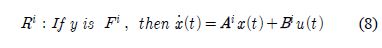
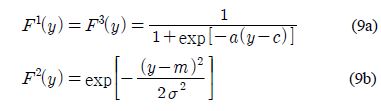
where Ai and Bi(i = 1, 2, 3) represent the system matrix and input vector of the corresponding operating point, respectively, and y represents the water level of the water tank. Also, for the antecedent fuzzy set, Fi (i=1,2,3), sigmoid type and Gaussian type were used as shown in Equation (9). F1 represents LO (Low), F2 represents MD (Medium), and F3 represents HI (High).
Figure 3 shows the antecedent fuzzy membership functions depending on the change in y using Equation (9).
The final output of the fuzzy model is inferred as shown in Equation (10) through weighted averaging.
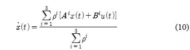
where ρi (i=1,2,3) is the contribution of the i-th membership function, and Fi(y) is the membership grade of the fuzzy set for the water level, y of the water tank.

Membership functions
2.3 Fuzzy-PID controller
The fuzzy combination of the output of the sub-PIDi (i=1,2,3) controller designed earlier is performed so that the parameters of the PID controller change depending on the change in the water level of the water tank system. Therefore, these can also be combined using an If-then rule, and can be expressed using the Takagi-Sugeno model similar to the method for obtaining the fuzzy model, as follows.
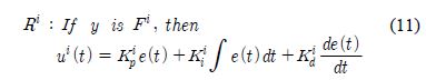
For the antecedent fuzzy set, Fi (i=1,2,3), the range of the water level is assumed to be from 4 [cm] to 12 [cm], and the fuzzy partitioning of the input space is performed using the membership functions that are identical to Figure 3. ui is the output of the sub-PIDi controller for the i-th rule. Kip, Kii(=Kip / Ti) and Kid (=Kip / Td)are the proportional gain, integral gain, and derivative gain of the sub-PIDi controller for the i-th rule, respectively.
Therefore, the output of the fuzzy-PID controller, uf , is inferred as follows.
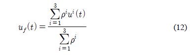
where ρi (i=1,2,3) is the contribution of the i-th membership function.
4. Simulation
4.1 Verification of the FOPTD estimation model
Before examining the performance of the proposed controller, the response characteristics of each estimated FOPTD model are verified. As shown in Figures 4~6, the estimated models are consistent with the submodels in the time domain and the frequency domain. In this regard, a slight disagreement is observed near the origin due to the time delay term of the FOPTD model.

Response characteristics of sub-MD1

Response characteristics of sub-MD2

Response characteristics of sub-MD3
4.2 PID controller
Figures 7~9 show the results of the simulation which was performed using the PID controller that had been designed based on the Z-N method, the C-C method, the IMC method, and the Lopez method using each estimated FOPTD model. As expected, the sub-PID controller designed at each submodel generally shows good response results. Especially, the GA-IAE method shows the highest performance considering the overshoot and the settling time.

Responses using sub-PID1 controller

Responses using sub-PID2 controller

Responses using sub-PID3 controller
4.3 Fuzzy-PID controller
Figure 10 shows the output responses of the two controllers in the fuzzy model, in order to compare the performances of the fuzzy-PID (F-PID) controller and the sub-PID controller. In this regard, the sub-PID controller has been tuned at sub-MD1 using the GA-IAE method, and shows the most outstanding response characteristics among the above four controller design methods.
As shown in the figure, the sub-PID controller shows outstanding performance at the operating point of 4 [cm] in the fuzzy model; but for the rest of the sections, satisfactory response is not obtained. However, the fuzzy-PID controller shows outstanding performance even in the fuzzy model where the parameters of the system change.

Comparison of the F-PID and sub-PID controller
5. Conclusion
In this study, a fuzzy-PID control technique for the level control of a single water tank system was proposed. In the proposed technique, for the water tank system, three linear submodels were obtained depending on the change in the water level. Then, a fuzzy model was implemented by combining them using a fuzzy rule. For the three submodels, FOPTD models were estimated using the least square error method; and based on this, each sub-PID controller was designed. Then, a fuzzy-PID controller that is capable of stable and effective control, was designed by combining them using a fuzzy rule.
The proposed technique showed outstanding adaptability and robustness when compared to the PID controller based on the simulation.
References
-
W. Grega, and A. Maciejczyk, “Digital control of a tank system”, IEEE Transaction on Education, 37(3), p271-276, (1994).
[https://doi.org/10.1109/13.312137]

- P. K. Kushwaha, and V. K. Giri, “PID controllers for water level control of two tank system”, International Journal of Electrical, Electronics & Communication Engineering, 3(8), p383-389, (2013).
- S. Nagammai, S. Latha, I. Aarifa, and S. D. Idhaya, “Analytical design of state feedback controllers for a nonlinear interacting tank process”, International Journal of Engineering and Advanced Technology, 2(4), p554-558, (2013).
- T. E. Rani, and J. S. Isaac, “Design of PI controller using characteristic ratio assignment method for coupled tank process”, Transactions on Engineering and Sciences, 1(4), p43-49, (2013).
- F. T. Abiodun, B. S. Habeeb, O. O. Mikail, and N. A. Wahab, “Control of a two layered coupled tank: Application of IMC, IMC-PI and pole-placement PI controllers”, International Journal of Multidisciplinary Sciences and Engineering, 4(11), p1-6, (2013).
- J. G. Ziegler, and N. B. Nichols, “Optimum setting for PID controllers”, Transactions of the American Society of Mechanical Engineers, 64, p759-768, (1942).
- G. H. Cohen, and G. A. Coon, “Theoretical investigation of retarded control”, Transactions of the American Society of Mechanical Engineers, 75, p827-834, (1953).
- M. Morari, and Z. Zafiriou, Robust Process Control, Prentice-Hall, Englewood Cliffs, (1989).
- A. M. Lopez, and C. L. Murill, “Tuning controller with error-integral criteria”, Instrumentation Technology, 14(2), p57-62, (1967).
- D. E. Kim, and G. G. Jin, “Model-based tuning rules of the PID controller using real-coded genetic algorithms", Journal of Control, Automation, and Systems Engineering, 8(12), p1056-1060, (2002).