Forecasting earning of VLCC tankers using artificial neural networks
Copyright © The Korean Society of Marine Engineering
This is an Open Access article distributed under the terms of the Creative Commons Attribution Non-Commercial License (http://creativecommons.org/licenses/by-nc/3.0), which permits unrestricted non-commercial use, distribution, and reproduction in any medium, provided the original work is properly cited.
Abstract
Shipping companies consistently want to minimize losses and maximize profits by accurately predicting the direction and magnitude of fluctuations in maritime situations. However, the determinants of maritime markets are diverse and volatile, and the decision mechanism is complex. Accurately predicting the direction and magnitude of fluctuations remains a difficult challenge. This study was conducted to evaluate the accuracy of multi-step-ahead forecasting of VLCC tanker markets by using an artificial neural network (ANN) training algorithm with the Levenberg-Marquardt and Bayesian regularization algorithms. The advanced time for forecasting was divided into one, three, six, nine, 12, and 15 months. The ANN predictions were conducted on the earnings for VLCC markets, and the datasets of the variables used in the forecast were 204 monthly time-series data from January 2000 to December 2016.
Keywords:
Artificial neural networks, VLCC, Forecasting1. Introduction
The world crude oil production in 2016 was 4448 million tons [1], and the total amount of crude oil transported by sea was 1949 million tons, which accounted for 43.8% of total crude oil production. The crude tanker demand for world seaborne trade was 178.5 million dwt for VLCC (200,000 dwt and over), 56.8 million dwt for SUEZMAX (125–199,999 dwt), and 55.5 million dwt for AFRAMAX (85–124,999 dwt) [2]. However, the oil tanker markets, which account for a large portion of world maritime transport, is highly influenced by the interaction of supply and demand in tanker transportation services and is highly volatile [3]. Therefore, predicting the changes in these markets is critical for all stakeholders, particularly those of the tanker market demand and supply sides.
This study focuses on predicting ANN for earnings for VLCC, which plays a major role in the marine transportation of crude oil. In addition, we evaluate the accuracy of an ANN prediction model when used with the Levenberg–Marquardt and Bayesian regularization algorithms.
Operating earnings can be derived from the time-charter rates or time-charter equivalent of spot rates when a vessel is operating in the spot market. Earnings are more representative of what an operating tanker produces [4]. Therefore, when choosing an ANN prediction target for the VLCC market, we selected the VLCC market earnings (USD/day) instead of the freight index (world scale, or WS).
2. Training algorithm of ANN
2.1 Mean squared error of ANN training algorithm
Learning is the fundamental capability of neural networks. Supervised learning adjusts network parameters by directly comparing the desired and actual network output. Supervised learning is a closed-loop feedback system in which the error is the feedback signal. The error measure, which indicates the difference between the output from the network and from training samples, is used to guide the learning process. The error measure is usually defined by the mean squared error (MSE) [5].
| (1) |
where Q is the number of pattern pairs in the sample set, tq is the output part of the qth pattern pair, and aq is the network output corresponding to the pattern pair q. The MSE is calculated anew after each epoch. The learning process is terminated when MSE is sufficiently small or the failure criterion is met.
2.2 Levenberg–Marquardt algorithm
The Levenberg–Marquardt algorithm, which is a numerical optimization technique [6], was designed to minimize functions that are sums of squares of other nonlinear functions in neural network training, where the performance index is the MSE.
When the performance index is F(x) , the Levenberg–Marquardt algorithm for optimizing the performance index F(x) is represented as [7]:
| (2) |
Here, as the changing value of μK, the performance index F(x) of the network can be adjusted through the optimization algorithms with a small learning rate, where J(xk) and V(xk) are the matrix elements used to compute the gradient.
2.3 Bayesian regularization algorithm
The complexity of a neural network is determined by the number of free parameters of weights and biases, which is determined by the number of neurons. If the network is too complex for a given dataset, then it is likely to overfit and have poor generalization [8]. The simplest method for improving generalization is early stopping. Another method is known as regularization [9]. One of two possible approaches can be used to improve the generalization capability of a neural network: restricting either the number of weights or the magnitude of weights, where the latter is called regularization.
The Bayesian regularization algorithm can be written as the sum of squares of network weights as follows:
| (3) |
where F(x) is the regularized performance index. Here, the regularization ratio α/β controls the effective complexity of the network solution.
3.Methodology
3.1 Data collection
The tanker freight market is characterized by interaction between many determinants of supply and demand in tanker transportation services [10]. To forecast the dynamics and fluctuations of freight rates in tanker freight markets, considerable research has been conducted using univariate or multivariate time-series analytical techniques [11] and ANN models [12].
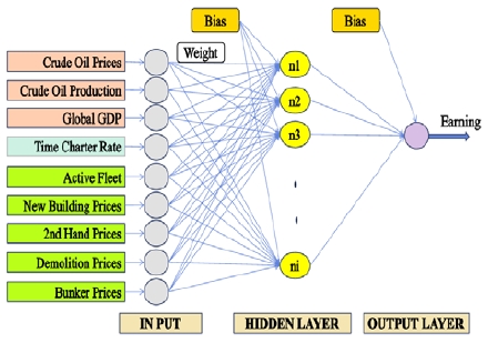
For all data used in forecasting of oil tanker markets in this study, global oil production, world GDP, active fleets, new building prices, second-hand ship prices, demolition prices, time-charter rates, bunker prices, and crude oil prices were selected as independent variables, whereas dirty tanker earnings was selected as the dependent variable.
Thus, the aggregated data were composed of nine independent variables and one dependent variable, where each variable was based on 204 monthly observations from January 2000 to December 2016.
3.2 Identification of ANN architecture
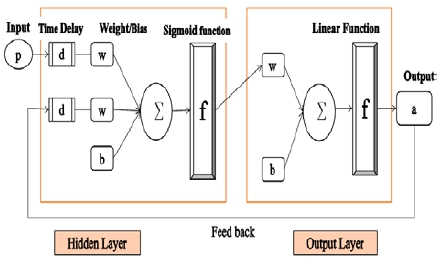
After the data for forecasting tanker markets were collected, the type of ANN architecture used to solve the problem of tanker market prediction, as well as the number of neurons and layers used in the network, were all determined. In ANN dynamic networks, the output depends not only on the current input to the network but also on previous inputs, outputs, and/or states of the network. Tanker markets prediction is part of an analysis that predicts the future value of a time series. Therefore, in this study, we selected dynamic networks as an appropriate ANN model to forecast dirty tanker markets. The non-linear autoregressive model with exogenous inputs (NARX networks) [5][8], which is a widely used network for applying predictions, is a recurrent dynamic network with feedback connections that encompass multiple layers of the network. This is shown in Figure 1.
Until now, prediction using ANN for VLCC tanker markets has been performed using the Levenberg–Marquardt training algorithm [12]-[15]. However, no Bayesian regularization algorithm has been used to predict earnings for such markets. Therefore, this study focuses on using ANN for prediction of earnings for VLCC tanker markets and evaluates the accuracy of the ANN prediction model using the Levenberg–Marquardt and Bayesian regularization algorithms.
After we identified the network structure, the number of hidden layers in these two learning algorithms was determined to enable us to compare performance results and functions more easily.
To determine the number of neurons in the hidden layer to identify the best prediction performance for the VLCC tanker market without overfitting, we adjusted the number of neurons in the hidden layer of the ANN structure using the Levenberg-Marquardt algorithm. In addition, using the Bayesian regularization algorithm, we had the ANN perform prediction for two cases using eight and 10 neurons of the hidden layer, respectively, based on nine total input variable numbers [7]. We then evaluated the performance results.
Only one neuron was present in the output layer, which had the same size as that of the target.
The prediction for VLCC markets earnings with the advanced periods of one, three, six, nine, 12, and 15 steps (months) were performed using MATLAB with the neural network toolbox. The inputs of the testing ANN model had nine nodes for input signals. In addition, the hidden layer was composed of neurons, with the tan-sigmoid transfer function selected as the neuron activation function. The value of the tagged delay line as a time delay was adjustable to avoid producing correlation effects.
3.3 Post-training validation
As an essential tool for neural network validation, the regression coefficient between the network output and target, known as the R value, should approximate 1 to ensure reliable ANN performance results. In addition, when applying dynamic networks for prediction, such as the focused time-delay neural network, two crucial factors must be considered when analyzing the trained prediction network: prediction errors should not be correlated either in time or with the input sequence.
4. Implementation
4.1 Data processing
The previously mentioned 204 data points of each variable in the period from January 2000 to December 2016 were randomly sampled during computation and divided into three datasets for training, validation, and testing. When the Levenberg–Marquardt algorithm was applied for iterative computing, the training set comprised approximately 70% of the full dataset, with the validation and test datasets each consisting of approximately 15%. In addition, when the Bayesian regularization training technique was applied, the testing data set was assigned as only 15% of the full dataset because the validation sequence was not applied to the algorithm.
4.2 ANN model for VLCC market prediction
A schematic of the ANN network for tanker market prediction is shown in Figure 2. When the Levenberg–Marquardt algorithm was applied, the number of neurons in the hidden layer was adjusted to improve the accuracy of the prediction performance. In addition, when the Bayesian regularization algorithm was applied, the number of neurons in the hidden layer was fixed to eight and 10 to compare the performance results of these two cases with those from the Levenberg–Marquardt algorithm.
The number of neurons in the output layer was the same as the size of the target. The output layer was composed of one neuron with the linear function as its activation function.
4.3 Computation
Each implementation for prediction was repeated several times to identify the optimal parameters and conditions of the network. When the results were unsatisfactory, training was repeated after weights and biases were initialized. When the Levenberg–Marquardt algorithm was trained, the number of neurons was adjusted to prevent overfitting or extrapolation. The value of the tagged delay line as a time delay was 2 (months) without any change made during implementation. The computational results from the Levenberg–Marquardt algorithm were considered as reasonable when the algorithm was fitted with the following considerations:
ㆍ The final mean performance index (MSE) was small
ㆍ The test set error (test performance index (MSE)) and validation set error (validation performance index (MSE)) had similar characteristics
ㆍ Expert judgment was used in determining various parameters and performance indices
When the Bayesian regularization technique was trained, 221 parameters in the 9-10-1 (input to number of neurons of the hidden layer to output) network, and 177 parameters in the 9-8-1 network were employed. The effective number of parameters was a minimum of 27 and a maximum of 172 when the 9-10-1 network was trained. The training of the 9-10-1 network effectively used less than 77% of the total number of weights and biases. The computational results for the training of the Bayesian regularization algorithm were considered as reasonable when the following were considered:
ㆍ The final mean performance index (MSE) was small
ㆍ The training error (training performance index (MSE)) was small
ㆍ Expert judgment was used in determining various parameters and performance indices
The computer used for the calculation had an Intel® Core ™ i5-5200U CPU @ 2.20 GHz.
4.4 Validation
The regression plots display the network outputs with respect to targets for training, validation, and test datasets. For this problem, the fit was reasonably good for all datasets, The validation for this problem was satisfactory for all data sets in each case with an R value of at least 0.93. The autocorrelation function of the prediction error and the cross-correlation function to measure the correlation between the input and prediction error were used during ANN prediction model validation.
5. Results
5.1 Comparison of prediction performance for VLCC
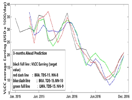
All implementation results of the mean performance index (MSE) are presented in Table 2 - Table 7 and Figure 3 - Figure 8 for use in evaluating the accuracy of the ANN prediction model.
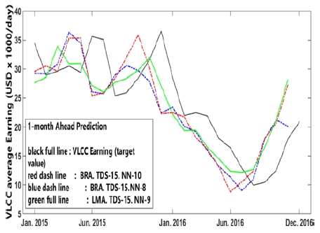
Figure 3 shows that BRA.TDS-15.NN-10 network had relatively good convergence with the total progression of the observation values . The networks of BRA.TDS-15.NN-10 and BRA.TDS-15.NN-8 showed better convergence-to-target values than did LMA.TDS-15.NN-9. The mean performance indices of the BRA.TDS-15.NN-8 and BRA.TDS-15.NN-10 networks were nearly the same. However, the training performance error of the BRA.TDS-15.NN-10 network was 0.266, which was much lower than that of the BRA.TDS-15.NN-8 network (1.3874), as shown in Table 2.
Table 1 shows the performance results for one-month-ahead prediction using the Levenberg–Marquardt algorithm for different numbers of neurons in the hidden layers. Each case shows best performance results without overfitting. When the number of neurons was greater or less than the number of input variables of 9, the results did not change satisfactorily. Note that during testing, the magnitude of the μ value was changed from 0.01 to 0.1 to speed up the conjugation.
Table 3 shows that with the Bayesian regularization algorithm, as the size of the hidden layer neuron increased, both the number of iterations and computing time increased, and the gradient value and train performance error (MSE) converged to a smaller value. However, even though the size of the hidden layer neuron increased in the short-term-ahead prediction, the mean performance index of 8.6425 for eight neurons showed significantly better results than 8.9288 for 10 neurons in the same forecasting horizon.
Table 4 shows that even though the number of hidden layer neurons increased from eight to 10 neurons, the gradient value and training performance error (MSE) did not converge to a smaller value. The training, validation, and test performance errors with the Levenberg–Marquardt algorithm showed a significant error in size despite no indication of overfitting or extrapolation.
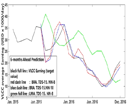
Figure 6 shows that the BRA.TDS-15.NN-8 network had relatively good convergence with the total progression of the observation values. However, during sudden up and down changes in the market, unstable prediction also appeared with the 6-months-ahead prediction. The training, validation, and test performance errors with the Levenberg–Marquardt algorithm showed significant errors in size despite no indication of overfitting or extrapolation.
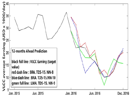
Table 6 shows that the mean performance index of 4.9389 with 10 neurons in 12-months-ahead prediction had better results than did the index of 9.3915 with eight neurons and as compared to the other training algorithm in the same forecasting horizon. As shown in the table, in the long-term-ahead forecasting, such as in 12-months-ahead prediction, the training algorithm, which had a larger hidden layer neuron, exhibited better forecasting performance than with the smaller neuron. The Levenberg–Marquardt algorithm showed a significant error in size despite no indication of overfitting or extrapolation.
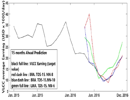
Table 7 shows that the mean performance index of 8.243 for 10 neurons with the Bayesian regularization algorithm generated better results than did the index of 10.5656 for eight neurons and as compared to the other training algorithm in the same forecasting horizon. As shown, similar performance results occurred with the 12-months-ahead prediction as with other long-term-ahead forecasting when the training algorithm was applied, where larger neurons exhibited better forecasting performance than did the smaller.
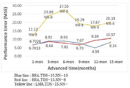
where:
LMA : Levenberg-Marquardt Algorithm
BRA : Bayesian Regularization Algorithm
TDS- : Test data set for full input data set (%)
NN- : Number of neurons of hidden layer
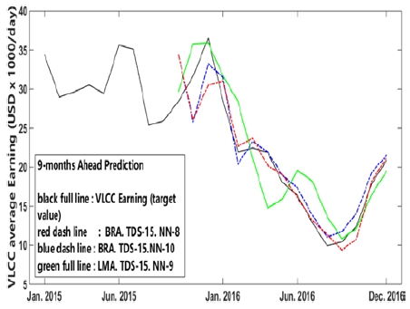
Figure 9 shows that the Bayesian regularization algorithm produced satisfactory results for all prediction horizons as compared to the Levenberg-Marquardt algorithm. In addition, in both training algorithms, the prediction results were generally satisfactory when the number of neurons in the hidden layer was similar to the number of input variables. The exception was 12-months-ahead prediction with the Levenberg-Marquardt algorithm. Particularly in the case of the Bayesian regularization algorithm, up to 9-months-ahead prediction showed more satisfactory prediction results with smaller neurons in the hidden layer as compared to the number of input variables. However, in 12- and 15-months-ahead predictions, results that are more satisfactory were obtained with greater numbers of neurons in the hidden layer as compared to the number of input variables.
6. Conclusion
In this study, we proposed alternatives to the ANN training algorithm to address the problem of multi-step forecasting. We used 204 monthly time-series data from 2000 to 2016 for dirty tankers of VLCC. Training algorithms used for the neural networks were the Levenberg–Marquardt and Bayesian regularization algorithms. A summary of this study’s findings are as follows.
ㆍ The Bayesian regularization algorithm outperformed the Levenberg-Marquardt algorithm for all prediction horizons.
ㆍ The prediction performance results from both algorithms were generally satisfactory when the number of neurons in the hidden layer was similar to the number of input variables.
ㆍ In the Bayesian regularization algorithm, when the size of the hidden layer neuron increased, the number of iterations and computing time increased, and the gradient value and training performance error (MSE) converged to a smaller value.
ㆍ In the predictions within 9-months-ahead prediction, the ANN training architecture with smaller neurons in the hidden layer showed the better performance.
ㆍ In the predictions exceeding 9-months-ahead prediction, the ANN training architecture with larger neurons in the hidden layer showed the better performance.
This study showed that ANN can be used as a major tool in more accurately predicting market changes regardless of the magnitude of fluctuations. However, to improve predictive performance, designing an optimal ANN architecture for predicting targets is essential.
Acknowledgments
This research was supported by Basic Science Research Program through the National Research Foundation of Korea (NRF) funded by the Korea Government (No.2017R1A2B2010603). Further, this has been also supported by the program of the developments of convergence technology funded by TIPA/SMBA of Korea (S2356988) and by the World Class 300 R&D program (S2415805), the Special Program for Occupation (R0006323) and Business Cooperated R&D Program (R000626) of MOTIE of Korean Government.
References
- The International Energy Agency (IEA), https://www.iea.org/statistics/kwes/ Accessed October 20, 2017.
- Clarksons Research Services, https://sin.clarksons.net/Timeseries Accessed December 19, 2017.
-
D. Hawdon, “Tanker freight rates in the short and long run”, Applied Economics, 10(3), p203-217, (1978).
[https://doi.org/10.1080/758527274]

-
A. H. Alizadeh, and N. K. Nomikos, “Trading strategies in the market for tankers”, Maritime Policy and Management, 33(2), p119-140, (2006).
[https://doi.org/10.1080/03088830600612799]

-
K. L. Du, and M. N. S. Swamy, Neural Networks and Statistical Learning, Springer, London, (2014).
[https://doi.org/10.1007/978-1-4471-5571-3]

- D. F. Shanno, Recent advances in numerical techniques for large scale optimization, Neural networks for control, Cambridge MA, MIT Press, (1990).
-
L. E. Scales, Introduction to Non-Linear Optimization, New York, Springer-Verlag, p110-136, (1985).
[https://doi.org/10.1007/978-1-349-17741-7]

- M. T. Hagan, H. B. Demuth, M. H. Beale, and O. D. Jesὑs, Neural Network Design, 2nd edition, (2014), [Online]. Available: http://hagan.okstate.edu/NNDesign.pdf.
- A. N. Tikhonov, “On the solution of ill-posed problems and the regularization method”, Dokl. Acad. Nauk USSR, 151(3), p501-504, (1963).
- M. Beenstock, and A. R. Vergottis, “An econometric model of the world tanker market”, Journal of Transport Economics and Policy, 23(2), p263-280, (1989).
-
M. G. Kavussanos, “Time varying risks among segments of the tanker freight markets”, Maritime Economics and Logistics, 5(3), p227-250, (2003).
[https://doi.org/10.1057/palgrave.mel.9100079]

-
J. Li, and M. G. Parsons, “Forecasting tanker freight rate using neural networks”, Maritime Policy and Management, 24(1), p9-30, (1997).
[https://doi.org/10.1080/03088839700000053]

-
P. Eslami, K. H. Jung, D. W. Lee, and A. Tjolleng, “Predicting tanker freight rates using parsimonious variables and a hybrid artificial neural network with an adaptive genetic algorithm”, Maritime Economics & Logistics, p1-13, (2016).
[https://doi.org/10.1057/mel.2016.1]

-
D. V. Lyridis, P. Zacharioudakis, P. Mitrou, and A. Mylonas, “Forecasting tanker market using artificial neural network”, Maritime Economics and Logistics, 6(2), p93-108, (2004).
[https://doi.org/10.1057/palgrave.mel.9100097]

-
A. Santos, L. N. Junkes, and F. C. M. Pires Jr, “Forecasting period charter rates of VLCC tankers through neural networks: A comparison of alternative approaches”, Maritime Economics & Logistics, 16(1), p72-91, (2013).
[https://doi.org/10.1057/mel.2013.20]


