A modified tabu search for redundancy allocation problem of complex systems of ships

1. Introduction

The RAP is a well-known combinatorial optimization problem which has been applied to reliability system designs such as semi-conductor integrated circuits, nanotechnology, and most electronic systems of ships, etc. The RAP is to determine the optimal number of redundant component in order to maximize the system reliability constrained to resource restrictions or system-level constraints for cost and weight. Many researchers have studied the RAP for various system structures of series, series-parallel, complex system, k-out-of-n, etc. Fyffe et al. [1] originallyset up the problem and suggested a solution algorithm utilizing a dynamic programming approach. Nakagawa and Miyazaki [2] developed 33 variations of Fyffe’s problem, where the weight constraint varied its value from 159 to 191. Coit and Liu [3] proposed zero-one integer programming for small size of problems. They constrained the solution space so that only the homogeneous component type can be allowed for each subsystem.

On the contrary, Coit and Smith [4] extended Fyffe’s problem in such a way that the parallel system could be more flexible. They allowed a mixing of component (i.e., heterogeneous component) types within a subsystem and employed GA (genetic algorithm) to obtain optimal solutions. RAP is usually formulated as a nonlinear integer programming problem which is generally difficult to find an exact optimal solution due to the considerable amount of computational effort. Therefore, various metaheuristic algorithms have been developed. Kultruel-Konak et al[5] developed TS (tabu search) algorithm for the RAP of series-parallel system, and it is hitherto known that solutions of Kultruel-Konak etal. [5] are the best among the other metaheuristics such as GA (Coit & Smith [4]), ACO (ant colony optimization; Liang & Smith [6]), VNS (variable neighborhood search; Liang & Chern [7]), and hybrid metaheuristics (Nahas et al. [8]). Recently, Ouzineb et al. [9] developed a hybrid metaheuristic which is combined TS with GA and obtained the same results of Kultruel-Konak et al. [5].

In the meanwhile, solutions for RAP of complex systems have been suggested by several authors (Ha & Kuo [10]). All authors have dealt with only the case of homogeneous components. In this paper, we suggest a RAPCH (RAP of complex systems with heterogeneous components) and find its optimal solution by the TS algorithm, the best in the literature. In addition, in order to enhance TS in terms of the quality of the solution, we develop a MTS (modified tabu search) to employ an adaptive mechanism combined with the TS. Computational results show that the proposed method obtains better results as the size of problem increases, even though it requires rather more computing time.

The rest of this paper is organized as follows. In Section 2, the model of RAPCH can be formulated as a nonlinear integer programming problem. In Section 3, we propose a MTS algorithm for the RAPCH to improve the quality of the solution of TS. In Section 4, a comparison of the case of the homogeneous components with that of the heterogeneous components is provided with an example, and in Section 5 we evaluate the performance of the proposed algorithm through the computational efforts. Finally, conclusions and future research are discussed in Section 6.

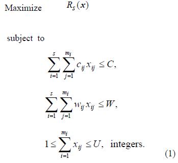
2. Statement of the problem

Notation

s    number of subsystems

x    the feasible solution

x₀      the initial feasible solution

x_c       the current solution

x_bf, x_binf    the best feasible or infeasible solution found so far

x_ij    the number of redundancy of the jth available component used in subsystem i

m_i    the number of available components for subsystem i

R_s(x)   the system reliability

R_i, Q_i     the reliability and unreliability of subsystem i

R_p(x)   the penalty function of the system reliability

C, W   system-level constraints limits for cost and weight

c_ij ,w_ij ,r_ij   the cost, weight and reliability for the jth available component for subsystem i

U      upper bound of x_ij

iter    the number of iterations of MTS

Adapiter  for adaptive procedure of MTS, the predetermined number of iterations without improving the value of R_s(x)

Stopiter   the maximum number of stopping iterations

Assumptions

In the RAPCH, assumptions are as follows:

  1. The system and all of its subsystems are s-coherent.

  2. The system consists of s subsystems, each of which is (1-out-of-x_ij: G).

  3. All component states are s-independent.

  4. Each constraint is an increasing function of x_ij and is additive among subsystems.

  5. System reliability R_s(x) is known in terms of the R_i.

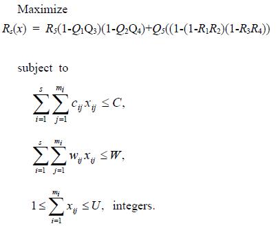
The RAPCH optimization model can be generally formulated as the following nonlinear integer programming problem:

This problem was proven to be a NP-hard problem (Chern [11]).

3. MTS Algorithm

To solve the RAPCH, we suggest a MTS to employ an adaptive procedure combined with the TS. The TS algorithm, first proposed by F. Glover [12], is a metaheuristic method to expand its search beyond local optimality using adaptive memory. The adaptive memory is a mechanism based on the tabu list of prohibited moves. The tabu list is one of the mechanisms to prevent cycling and guide the search towards unexplored region of the solution space. TS generally adopts the penalty function to allow to explore the search towards the promising infeasible region. The TS has been successfully applied to many combinatorial optimization problems such as ship routing problems, traveling salesman problems, time tabling problems, and resource allocation problems, etc.

Our MTS is based on the TS of Kultruel-Konak et al. [5]. The MTS consists of four parts which are i) construction of initial solutions and stopping criterion, ii) tabu list, iii) the structure of generating the neighborhood solutions, and iv) penalty function. Among them, iii) the structure of generating the neighborhood solutions is usually different according to the characteristics of the decision variables for the problem. The general steps of MTS can be summarized as follows:

Step 0. (Initialization) Set iter=0,and initialize tabu list.

Step 1. Randomly generate the initial solution x₀. Set x_c = x₀ and x_bf = x_binf = x_c.

Step 2.a. (Adaptive procedure)

     Set iter = iter+1.

     If iter ≤ Adapiter, generate the neighborhood of xc by the 1-opt exchange.

     Otherwise, generate the neighborhood of x_c by the 2-opt exchange (see [13]).

Step 2.b. Select the best neighborhood which is not in the tabu list. Store it as the new current solution. Update the tabu list.

Step 3. If x_c is feasible, then go to step 4. Else go to step 5.

Step 4. If R_s(x_c) > R_s(x_bf), then set x_bf = x_c, iter = 0, and initialize the tabu list. Go to step 2.a. Else go to step 6.

Step 5. If R_p(x_c) > R_s(x_binf), then x_binf = x_c, iter = 0, and initialize the tabu list. Go to step 2.a.

Step 6. If iter > Stopiter, then goto step 7. Else go to Step 2.a.

Step 7. (End) Stop with the best feasible solution found so far.

3.4 Penalty function

The MTS generally adopts the penalty function to allow to explore the search towards the promising infeasible region. The penalty function of Kultruel-Konak et al. [5] is adopted in our MTS. The penalty function for two independent constraints (cost and weight) is as follows:

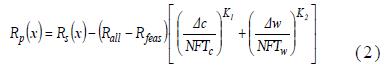
where R_all is the unpenalized (feasible or infeasible) system reliability of the best solution found so far, R_feas is the system reliability of the best feasible solution found so far, and ∆c and ∆w represent the magnitude for the violation of the cost and weight constraint, respectively. The initial values of NFT_c and NFT_w are set to 1% of the constraint limit for the cost and weight, respectively. The values of K₁ and K₂ are set to 1, though computational results are insensitive to these values.

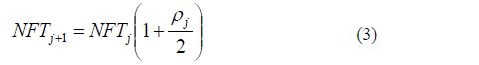
The value of NFT_j at any given iteration j is updated as follows. If the current move is to a feasible solution, then

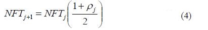
If the current move is to a infeasible solution, then

where ρ_j, a feasibility ratio at iteration j, is defined as

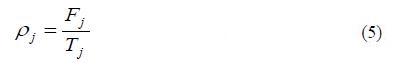
The tabu list size at any given iteration j is defined as T_j, and the number of feasible solutions on the current tabu list is defined as F_j. The value of NFT changes according to the count of the feasible versus infeasible solutions on the tabulist. If the current move is feasible, Eq. (3) has a property of encouraging the search toward the promising infeasible regions. That is, this decreases the penalty for an infeasible solution and moves the search toward the infeasible region. Reversely, if the current move is infeasible, Eq. (4) increases the penalty for an infeasible solution and explores the search backward the feasible region.

4. An Example

We suggest an example of RAPCH in this paper. The system structure and subsystem data are given by Figure 1 and Table 1, respectively.

Figure 1:

A bridge network system

The RAPCH is formulated as follows:

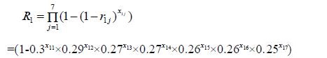
For example, R₁ is given by

When C = 34 and W = 51 of this RAPCH, the TS yields an optimal solution, that is, x₁₁ = x₂₁ = x₂₂ = x₃₆ = x₃₇ = x₄₁ = x₄₅ = x₅₂ = 1, R_s(x) = 0.981432. The heterogeneous structure of this solution is shown in Figure 2(b).

Figure 2:

The optimal solutions for homogeneous and heterogeneous components

In Figure 2(a), the optimal solution for the case of homogeneous components is given by x₁₃ = 1, x₅₂ = 1, x₂₂ = 1, x₃₇ = 1, x₄₁ = 1, R_s(x) = 0.980906. This result indicates that the design of heterogeneous components can provide the possibility of having the better system reliability than that of homogeneous components.

5. Computational Experiments

To additionally evaluate the performance of the TS and the proposed MTS, test problems for moderate size of system structure are designed. They are composed of 3 sets of 10 test problems, that is, 30 test problems totally. We replicated the data in Table 1 by h-hold, where h ranges from 6, 8 to 10, i.e., the number of subsystems of each problem became s = 5 × h (i.e., 30, 40, 50).

Table 1:

Input data for heterogeneous components of bridge network system

As mentioned in section 3, TS generally adopts 1-opt exchange procedure as a strategy of generating the neighborhood solutions. It is apt to be trapped in a local optimum, regardless of the considerable amount of exploring solutions. In order to alleviate the risks of being trapped in such a local optimum, the adaptive procedure of alternatively allowing 2-opt exchange procedure of generating the neighborhood solutions is employed in MTS, even though it requires rather more computing time. That is, our MTS exploits 1-opt exchange procedure at the first predetermined Adapiter iterations, and then adopts 2-opt exchange procedure after the Adapiter iterations to escape the local optimum.

At first, in order to determine the proper value of Adapiter as the flexible strategy of generating the neighborhood solutions of our MTS algorithm, we performed a sensitivity analysis for stopping criterion of TS. We varied the value of Stopiter from 100, 500 to 1000.

We compared their performance by extending the size of subsystem from 30 up to 50. From our computational experiments, we noticed that the compromised number of Adapiter (i.e., the end phase of the 1-opt exchange) was 500. As a result, MTS employs the 1-opt exchange at the first 500 iterations without improving Rs(x), and then adopts the 2-opt exchange after the 500 iterations without improving R_s(x). The computational results of sensitivity analysis for stopping criterion are shown in Table 2. Among TS(100), TS(500), and TS(1000), the TS(1000) obtains the best results in terms of solution quality. However, it requires the considerable amount of computing time. The performance of our MTS is also shown in the last column of Table 2. From Table 2, we notice that our MTS obtains the better solution in 2, 5 and 8 cases for s=30, 40 and 50, respectively than the TS(1000). From the computational results, we notice that the proposed method obtains the better results than the TS, as the size of the problem increases from 30 to 50, even though MTS requires rather more computing time than the TS.

Table 2:

A comparison of TS and MTS(a) s=30

(b) s=40

(c) s=50

6. Conclusions

Solutions for RAP of complex systems have been suggested by several authors (Ha & Kuo [10]). All authors have dealt with only the case of homogeneous components. In this paper, we suggested a RAP of complex systems with heterogeneous components and obtained its optimal solution by the TS algorithm which is the best in the literature. In addition, in order to enhance TS in terms of the quality of the solution, we developed a MTS to employ an adaptive procedure (1-opt or 2-opt exchange) combined with the TS. Computational results showed that the proposed method obtained the better results as the size of the problem increases, even though it requires rather more computing time.

To improve the quality of the solution, the development of more powerful metaheuristics for the RAPCH should be performed in future research. With some adjustment of the parameters of the proposed method, it can be applied to the optimal reliability designs of complex systems of ships.

References

• D. E. Fyffe, W. W. Hines, and N. K. Lee, “System reliability allocation and a computational algorithm”, IEEE Transactions on Reliability, 17, p64-69, (1968). [https://doi.org/10.1109/TR.1968.5217517]
• Y. Nakagawa, and S. Miyazaki, “Surrogate constraints algorithm for reliability optimiza- tion problems with two constraints”, IEEE Transactions on Reliability, 30, p175-180, (1981).
• D. E. Coit, and J. Liu, “System reliability optimization with k-out-of-n subsystems”, International Journal of Reliability, Quality and Safety Engineering, 7, p129-142, (2000). [https://doi.org/10.1142/S0218539300000110]
• D. W. Coit, and A. E. Smith, “Reliability optimization of series-parallel systems using a genetic algorithm”, IEEE Transactions on Reliability, 45, p254-260, (1996). [https://doi.org/10.1109/24.510811]
• S. Kulturel-Konak, B. A. Norman, D. W. Coit, and A. E. Smith, “Exploiting tabu search memory in constrained problems”, INFOR- MS Journal on Computing, 16, p241-254, (2004). [https://doi.org/10.1287/ijoc.1030.0040]
• Y. C. Liang, and A. E. Smith, “An ant colony optimization algorithm for the reliability allocation problem (RAP)”, IEEE Transactions on Reliability, 53, p417-423, (2004).
• Y. C. Liang, and Y. C. Chen, “Redundancy allocation of series-parallel systems using a variable neighborhood search algorithm”, Reliability Engineering and System Safety, 92, p323-331, (2007). [https://doi.org/10.1016/j.ress.2006.04.013]
• N. Nahas, M. Nourelfath, and D. Ait-Kadi, “Coupling ant colony and the degraded ceiling algorithm for the redundancy alloca- tion problem of series-parallel systems”, Reliability Engineering and System Safety, 92, p211-222, (2007).
• M. Ouzineb, M. Nourelfath, and M. Gendreau, “An efficient heuristic for reliability design optimization problems”, Computers & Operations Research, 37, p223-235, (2010). [https://doi.org/10.1016/j.cor.2009.04.011]
• C. Ha, and W. Kuo, “Initial allocation compensation algorithm for redundancy allocation: The scanning heuristic”, IIE Transactions, 40, p678-689, (2008). [https://doi.org/10.1080/07408170701730800]
• M. S. Chern, “On the computational complexity of reliability redundancy allocation in a series system”, Operations Research Letters, 11, p309-315, (1992). [https://doi.org/10.1016/0167-6377(92)90008-Q]
• F. Glover, “Future Paths for Integer Programming and Links to Artificial Intelligence”, Computers and Operations Research, 13, p533-549, (1986). [https://doi.org/10.1016/0305-0548(86)90048-1]
• J. Renaud, F. F. Boctor, and J. Ouenniche, “A heuristic for the pick up and delivery traveling salesman problem”, Computers and Operations Research, 27, p905-916, (2000).