
Analysis of haline channel formed in the East China Sea and the Atlantic Ocean using the T-S gradient diagram
In case of any coastal ocean near the mouth of huge rivers, low salinity water can be formed due to its large amount of freshwater discharge. For the acoustic analysis on the low salinity environment, some oceanographic data of the East China Sea and the Atlantic Ocean were collected through KODC (Korea Oceanographic Data Center) and NODC (National Oceanographic Data Center) online service. In this paper, the T-S gradient diagram is introduced to show a relation between the gradients of temperature and salinity in view of acoustic surface channel formation. Existence of haline channel, quantitative contribution of gradients of salinity and temperature, effectiveness of the channel formation can be known by the T-S gradient diagram. After applying the collected data into the diagram, tropical regions of the Atlantic Ocean show strong haline channel due to its nearly invariant temperature and drastic change of salinity with depth. The averaged transmission loss in the channel is about 5.7 ~ 7.5 dB less than that out of the channel by the results of acoustic propagation model (RAM: Range independent Acoustic Model). On the other hand, the East China Sea and temperate region of the Atlantic ocean have weaker haline channel with less difference of the averaged transmission loss between in and out of the channel as 3.2 ~ 6.0 dB. Although data samples used in this study have limitation to represent the general physical structures of the three ocean regions, the T-S gradient diagram is shown to be useful and acoustic field affected by low salinity environment is investigated in this study.
Keywords:
Haline channel, Low-salinity, T-S gradient diagram, RAM model1. Introduction
Temperature, salinity, and hydrodynamic pressure affect sound speed in the ocean. Among them, water temperature and pressure dynamically change with depth and give more influence on the sound speed variation than salinity. Salinity not only has weak contribution to sound speed, but also shows small spatial variation. Hence, it is mostly disregarded in the sound speed calculation [1].
However, low salinity water freshened by some other facts is sometimes observed at the coastal oceans. In this case, the effects of salinity may not be negligible in the calculation of sound speed, so that we may need to carefully consider its effects on sound speed and sound propagation in the oceans.
According to oceanographic studies on low salinity water, ocean water is mainly freshened by continental runoff, precipitation over the sea surface, and advection of fresh waters from large flows. In particular, the fresh water discharges from huge rivers are the most influential factor among them [2]-[6]. In case of the western sea of Jeju island, ocean water whose salinity less than 30 psu is called low salinity water [7].
While many oceanographic researchers have investigated the low salinity water at many coastal oceans, only a few acoustic investigations have been performed.
Dosso and Chapman studied sound propagation in a shallow sound channel in the northeast Pacific Ocean [8]. They studied sound propagation in the channel by analyzing transmission loss with frequency but they did not deal with the channel formation process in the low salinity environment.
Bulgakov et al. reported that highly freshened surface water in the tropical Atlantic Ocean reduces sound speed and, thereby, forms a haline channel which is an acoustic surface channel formed mainly by salinity [9]. They distinguished it from hydrostatic channel, which is more affected by hydrostatic pressure than by either temperature or salinity. However, their study is limited to explain the channel formation process in low salinity environment in detail.
Recently, we explored the sound speed variation in low salinity water with haline channel formation in the western sea of Jeju island [10]. According to the results, more than half of measured low salinity waters form haline channels but there are also many exceptional cases that the channel was not formed even in very low salinity water. Sometimes, it is not clear enough to explain the cause of channel formation by only vertical profiles of temperature and salinity. Therefore, another approach is needed to find additional causes of haline channel formation.
In order to study the condition for haline channel formation, a T-S gradient diagram is introduced in this paper. It presents a relation between the gradient of temperature and that of salinity to compare minimum requirement for formation of an acoustic surface channel. The oceanographic data are applied into the diagram to confirm a usefulness of the diagram. In addition, transmission loss is calculated in low salinity environment by an acoustic propagation model based on parabolic wave equation to study acoustic characteristics.
2. Data
2.1 Data acquisition sites
Low salinity water in the ocean is formed by many reasons, but discharge of fresh water is the most influential factor to form low salinity waters. Therefore, three sites close to the mouth of huge rivers were selected in order to collect the oceanographic data in low salinity environment.
The first site is on the East China Sea nearby the Jeju Island [P: 33.0°N, 125.0°E] (Figure 1 (a)). The low salinity water in the East China Sea is formed by discharge of the Yangtze River all year round. But, in particular, it spreads out to the East by the south wind in summer so that it reaches the Yellow Sea.

Location of data acquisition sites: (a) a measurement site near the Yangtze River in the East China Sea, (b) two regions of interest in the Atlantic Ocean near South America, (c) two sites near the mouth of Amazon River on equator region of the West Atlantic Ocean, (d) two sites near the mouth of La Plata River on Southwest Atlantic Ocean
The second site is on the tropical region of western Atlantic Ocean. Surface salinity in that region is strongly affected by the Amazon River. One of the biggest rivers in the world discharges large amount of fresh water into the ocean. Two different sites near the mouth of Amazon River were selected [A1: 3.9528°N, 50.0364°W and A2: 5.3630°N, 50.9000°W].
Lastly, the other site in the southwest area of the Atlantic Ocean is selected [B1: -36.503°S, 53.762°W and B2: 54.6501°S, 36.3084°W]. The mouth of La Plata River (Rio de La Plata) discharges large amount of fresh water
The NODC (National Oceanographic Data Center, USA) integrates various oceanographic data measured by many other countries and provides it through online service [11]. In order to download the data set corresponding to the regions of interest in this study, WOD09 (World Ocean Database 2009) with OSD (Ocean Station Data), CTD data were selected in the website. Those are used for analysis of the Atlantic Ocean. For the East China Sea, KODC (Korea Oceanographic Data Center) data is used [12].
2.2 Vertical profiles of physical properties
After the survey on massive amount of oceanographic data to find the appearance of low salinity water, some representative data sets were selected for this study. Among some oceanographic data, temperature and salinity at certain depth were used to calculate sound speed. Figure 2 shows some vertical profiles of temperature, salinity and sound speed measured on August in1996, 2002 and 2003 at the site P (Figure 1 (a)).

Temperature, salinity and sound speed profile of site P (in East China Sea). Case 1: normal salinity, case 2: low-salinity case with haline channel, case 3: low-salinity case with no channel.
The profiles of temperature in Figure 2 (a) show typical structures of the region of site P in summer with a weak mixed layer and strong thermocline. On the other hand, they have all different types of salinity profiles as shown in Figure 2 (b).
The case 1 measured on 4 Aug 2002 shows 30.63 psu of surface salinity and gradual gradient with depth (dash-dot line in Figure 2 (b)). It is presented as a normal salinity structure for comparison with two other low salinity cases. In case 2 measured on 5 Aug 1996, the low salinity water was formed near surface. Its surface salinity was very low (21.35 psu) and it shows sharp increase with depth (dashed line in Figure 2). Consequently, the haline channel was formed near surface. The gradient inversion of sound speed is observed in Figure 2 (c). On the other hand, while the surface salinity was low as 25.69 psu and it steeply increased with depth as shown in Figure 2 (b) (solid line, case 3), there was no haline channel formed near surface. Its sound speed profile was more similar trend to normal salinity case rather than the low salinity water case.
The other oceanographic data measured in two different regions of the Atlantic Ocean were also analyzed. Since these data were selected to show the low salinity environment as examples, it dose not fully represent the physical structure of these regions.
The equator region on the Atlantic Ocean usually has a thick mixed layer resulted from the consistently warm climate. Figure 3 (a) shows a well-developed mixed layer with relatively weak thermocline. Meanwhile, it shows very low salinity on the surface by the fresh water from the Amazon River. It was 23.69 psu and 26.83 psu in the site A1 on 19 Mar. 1995 and A2 on 10 Apr. 1999 respectively (Figure 3 (b)). Since the influence of temperature on sound speed variation with depth is tenuous, the drastic change of salinity near surface can strongly affect sound speed variation with depth.

Temperature, salinity and sound speed profile of site A1 (dashed line) and site A2 (solid line) (in equator region of western Atlantic Ocean near the mouth of Amazon River).
Since the sound speed decrease from the surface it has a sharp incline with depth. Hence, the haline channel was formed (Figure 3 (c)).
Since the strong current flows along the coastline in the outer shelf in the region B (Figure 1 (d)), the discharge of fresh water from the La Plata River affects surface salinity mainly in the continental shelf [3]. Site B1 and B2 are near the border of the shelf so that the surface salinity is not much lower than the other cases. Meanwhile, the temperature structures are composed of a mixed layer with thermocline and it shows seasonal variation of sea surface temperature due to temperate climate (Figure 4 (a)). Although these were measured in different seasons, the surface channel was formed in both cases with small positive sound speed gradients by the low salinity water as shown in Figure 5 (b) and (c).

Temperature, salinity and sound speed profile of site B1 (dashed line) and site B2 (solid line) (in southwest Atlantic Ocean near the mouth of La Plata River).

The results of T-S gradient diagrams for East China Sea (a) normal salinity environment in 2002 (b) low salinity environment with haline channel in 1996, (c) low salinity environment with no channel in 2003
3. Methodology
3.1 T-S gradient diagram
The low salinity of ocean surface is not the only a factor to form a haline channel. It can be inferred from the profiles in case 3 as shown in Figure 2 (solid line). Even though the surface salinity was very low, the haline channel was not formed. Therefore, various data were analyzed for inductive reasoning and, finally, the gradients of temperature and salinity were considered as important factors for haline channel formation.
The acoustic channel is related by sound speed variation with depth in the ocean. Hence, in order to get a gradient of sound speed, a formula by Medwin is used [13].
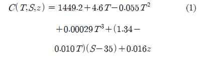
In case of the surface channel, it can be formed by positive gradient of sound speed.
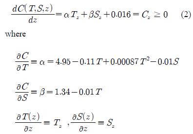
Tz and Sz are temperature and salinity gradients with depth, respectively. The influence of salinity is much smaller than that of temperature in α, so it can be disregarded. Then, α, β are functions of temperature alone. Hence, this formula can be rearranged as
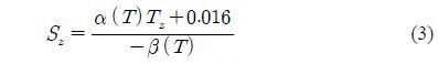
where Cz is considered as zero. Equation (3) indicates a relation of Tz and Sz. When T and Tz are given at a certain depth, a minimum value of Sz required for channel formation can be calculated by using Equation (3). We can decide whether a surface channel is formed or not, by comparing the measurement gradients with the calculated minimum gradients for channel formation. Both values of Tz and Sz can be presented in a 2D diagram. This diagram is called T–S gradient diagram in this paper. To satisfy the channel formation condition, the gradients of measurement data should exceed the line of minimum gradients (threshold line).
3.2 Transmission Loss
For the more study on acoustic propagation in the low salinity environment, acoustic analysis is conducted using an RAM (Range-dependent Acoustic Model) based on parabolic wave equation modeling [14]. Flat ocean surface and bottom with range independent environment are assumed for this simulation. A radiation frequency of an acoustic source was 5 kHz and its location was 3m and 6m from a surface for the East China Sea and the Atlantic Ocean, respectively, considering the channel depth. Sound speed and density of sea-bed were 1650 m/s and 1900 kg/m3, respectively.
4. Results
4.1 The East China Sea
The results of the T-S gradient diagram analysis are shown in Figure 5 for the East China Sea. The circles in the diagrams represent measurement gradients of temperature and salinity at certain depths; they have a 1m depth interval from 0m to 20m (the two boundaries are marked with a triangle and a square, respectively). Since the slops of threshold line slightly varies with depth by temperature (Equation (3)), the median line (10m) was selected representatively.
Figure 5 (a) shows the result of a normal salinity environment in 2002 of the East China Sea. All measurement gradients are under the threshold line. It means that the ocean physical structure does not form the channel. Otherwise, some of gradients are above the threshold line in low salinity environment in 1996 (Figure 5 (b)). The gradients of temperature with depth in 1996 are not much different from those in 2002 but the gradients of salinity are much higher. Due to the high values of salinity gradients, it exceeds the threshold line.
While it was not clear to understand the reason why there was not haline channel even in low salinity environment in 2003 by the vertical profiles of temperature and salinity (Figure 2, solid line), the reason can be clearly explained through Figure 5 (c). The gradient of salinity was high in case of 1996 but the drastic decline of temperature with depth (high negative gradient of temperature) interrupts it to form a haline channel.
When the haline channel is formed, the acoustic field greatly changes in terms of transmission loss. Less transmission loss is shown along the surface in low salinity environment with the haline channel formation in Figure 6 (a). On the other hand, when the haline channel was not formed, even in low salinity environment, transmission loss is not much decreased along the surface in Figure 6 (b). It can be confirmed more clearly using vertical line transmission losses.
Mean vertical transmission loss over the ranges of 1500 m and 2500 m is shown in Figure 7. The less transmission loss in the channel is clearly indicated by Figure 7 (a) and (b).

Transmission loss of acoustic propagation (a) low salinity environment with haline channel near sea surface in 1996, (b) low salinity environment with no channel in 2003.

Vertical line transmission loss at range 1500m. (a) low salinity environment with haline channel near sea surface in 1996, (b) low salinity environment with no channel in 2003.
After averaging the mean vertical losses both above 10m and bellow 10m, they were 54.0 dB and 59.4 dB, respectively, and their difference is 5.4 dB in the haline channel environment (Figure 7 (a)). On the other hand, in the non-haline channel environment, they were 55.4 dB and 59.0 dB, respectively, and it shows less difference of vertical transmission loss (3.6 dB) than the case of haline channel formation (Figure 7 (b)).
4.2 The Atlantic Oceans
Due to the nearly zero gradient of temperature by well-developed mixed layer in tropical Atlantic Ocean, the gradient of salinity gives large influence on haline channel formation as shown in Figure 8. While there are very small temperature gradients, the gradients of salinity get high value with depth.

The results of the T-S gradient diagrams for the tropical Atlantic Ocean near the mouth of the Amazon River of South America (a) gradients of temperature and salinity measurement data at site A1 in Mar 1995 (b) gradients of temperature and salinity measurement data at site A2 in Apr 1999
Therefore, the results of Figure 8 whose marker positions are far from threshold line show that the haline channel was strongly formed in those environments. It is also shown in Figure 9. The acoustic channel is formed along the sea surface with less transmission loss. When we compare the averaged vertical line transmission losses along the range, it is smaller in the channel than out of the channel as 5.0 dB at site A1 and 4.9 dB at site A2.

Transmission loss in tropical Atlantic Ocean near the mouth of Amazon River of South America (a) site A1 on Mar, 1995, (b) site A2 on Apr, 1999.
The southwest region of the Atlantic Ocean near the mouth of the La Plata River has temperate climate so that it has a mixed layer and a thermocline which varies with seasons. Therefore the gradients of temperature are somewhat changed with depth. The gradients of salinity also changed with depth.
However, an influence of the salinity gradients on sound speed slightly surpasses that of temperature gradient so that the haline channel was formed. As shown in Figure 11, the haline channel was formed with less transmission losses along the surface but it has not large difference as much as the tropical region of Atlantic Ocean. The averaged transmission loss in the channel is less than that out of the channel as 4.4 dB and 3.2 dB at site B1 and B2, respectively.

The results of T-S gradient diagrams for sub-tropical Atlantic Ocean near the mouth of La Plata River of South America (a) gradients of temperature and salinity measurement data at site B1 on Dec. 1989 (b) gradients of temperature and salinity measurement data at site B2 on Aug. 1991

Transmission loss in sub-tropical Atlantic Ocean near the mouth of La Plata River of South America (a) site A1 on Mar, 1995, (b) site A2 on Apr, 1999.
5. Conclusion
Many oceanographic researches on the low salinity water formed in coastal ocean near huge rivers have been conducted. However, acoustic studies were not much investigated yet. In order to know the acoustic characteristics in low salinity water, several approaches were introduced in this paper.
The most important phenomenon in low salinity environment is a formation of haline channel. Once the channel is formed, spatial acoustic field changes because some of acoustic energy propagates along the channel. One of reasons for the formation of haline channel is the low salinity which makes the sound speed lower so that the gradients of sound speed can be positive. However, in some environment, the haline channel is not formed even the surface salinity is very low. In order to analyze the many different cases regarding haline channel formation, the T-S gradient diagram is introduced in this paper. It is based on the relation between the gradient of temperature and that of salinity satisfying the minimum requirement for formation of an acoustic surface sound channel. Some cases of measurement data of the East China Sea and the Atlantic Ocean were applied to confirm the diagram. One case of measurement data showed that the haline channel was not formed even in the low salinity water. After using the T-S gradient diagram, it was clearly explained that the negative gradient of temperature interrupt formation of a haline channel. Furthermore, transmission loss for each case was simulated to study acoustic propagation in low salinity water. When the low salinity water fail to form a haline channel, the transmission loss distribution in space was not much changed and similar to that in normal salinity water. However, if the low salinity water forms a haline channel, the transmission loss fields change significantly. In particular, the transmission loss decreased as around 6 dB along the channel.
Two regions in the Atlantic Ocean were also analyzed. In case of the tropical region near the mouth of the Amazon River, the gradients of temperature and salinity were far above the threshold line which represents the minimum condition of channel formation theoretically due to the nearly invariant temperature and sharp increase of salinity with depth. It means that the haline channel was strongly formed, which was also confirmed by the simulation of acoustic propagation.
On the other hand, temperate coastal area of Atlantic Ocean near the mouth of the La Plata River showed weaker channel due to the gradual salinity changes with depth (it is shown in T-S gradient diagram close to the threshold line).
Data samples used in this study were limited to represent the ocean physical structures of the three regions. The usefulness of the suggested T-S gradient diagram and acoustic filed change corresponding to each low salinity environment are emphasized and introduced in this study. In order to better understand sound propagation in haline channel, more systematic acoustic analysis including frequency dependency of transmission loss through the channel needs to be studied.
Acknowledgments
This research was supported by the 2013 scientific promotion program funded by Jeju National University
Notes
References
- T. U. Bhaskar, D. Swain, and M. Ravichandran, “Seasonal variability of sonic layer depth in the central arabian sea”, Journal of Ocean Science, 43(3), p147-152, (2008).
-
J. Salisbury, D. Vandemark, J. Campbell, C. Hunt, D. Wisser, and N. Reul, “Spatial and temporal coherence between Amazon River discharge, salinity, and light absorption by colored organic carbon in western tropical Atlantic surface waters”, Journal of Geophysical Research, vol. 116 (C00H02), p1-14, (2011).
[https://doi.org/10.1029/2011JC006989]

-
E. D. Palma, R. P. Matano, and A. R. Piola, “A numerical study of the Southwestern Atlantic Shelf circulation: Barotropic response to tidal and wind forcing”, Journal of Geophysical Research, vol. 109 (C08014), p1-17, (2004).
[https://doi.org/10.1029/2004JC002315]
-
N. S. Banas, P. MacCready, and B. M. Hickey, “The Columbia River plume as cross-shelf exporter and along-coast barrier”, Continental Shelf Research, 29, p292-301, (2009).
[https://doi.org/10.1016/j.csr.2008.03.011]
-
R. C. Beardsley, R. Limeburner, H. Yu, and G. A. Cannon, “Discharge of the Changjiang (Yangtze River) into the East China Sea”, Continental Shelf Research, 4(1), p57-76, (1985).
[https://doi.org/10.1016/0278-4343(85)90022-6]
-
P. C. Fiedler, and L. D. Talley, “Hydrography of the eastern tropical Pacific: A review”, Progress in Oceanography, 69, p143-180, (2006).
[https://doi.org/10.1016/j.pocean.2006.03.008]
- K. H. Oh, Y. G. Park, D. I. Lim, H. S. Jung, and J. S. Shin, “Characteristics of temperature and salinity observed at the Ieodo ocean research station”, Journal of the Korean Society for Marine Environmental Engineering, 9(4), p225-234, (2006), (in Korean).
- S. E. Dosso, and N. R. Chapman, “Acoustic propagation in a shallow sound channel in the Northeast Pacific Ocean”, Journal of the Acoustical Society of America, 75(2), p141-147, (1992).
-
N. P. Bulgakov, Y. V. Artamonov, P. D. Lomakin, and V. N. Cheremin, “Acoustic properties of surface water masses in the tropical Atlantic and their seasonal variability”, Soviet Journal of Physical Oceanography, 3(2), p141-147, (1992).
[https://doi.org/10.1007/BF02197620]
-
J. Kim, T. H. Bok, D. G. Paeng, I. C. Pang, and C. Lee, “Acoustic channel formation and sound speed variation by low-salinity water in the western sea of Jeju during summer”, Journal of the Acoustical Society of Korea, 32(1), p1-13, (2013).
[https://doi.org/10.7776/ASK.2013.32.1.001]
- NODC (National Oceanographic Data Center), www.nodc.moaa.gov/OC5/SELECT/dbsearch/ dbsearch.thml.
- KODC (Korea Oceanographic Data Center), http://kodc.nfrdi.re.kr.
-
H. Medwin, “Speed of sound in water: A simple Equation for realistic parameters”, Journal of the Acoustical Society of America, 58(6), p1318-1319, (1975).
[https://doi.org/10.1121/1.380790]
- M. D. Collins, “Users Guide for RAM Versions 1.0 and 1.0p”, ftp://ftp.apl.washington.edu/archive/whales/Haro_Strait /rrsfc/ram.pdf, Acessed November 9, 2013.