A nonlinear transformation methods for GMM to improve over-smoothing effect
We propose nonlinear GMM-based transformation functions in an attempt to deal with the over-smoothing effects of linear transformation for voice processing. The proposed methods adopt RBF networks as a local transformation function to overcome the drawbacks of global nonlinear transformation functions. In order to obtain high-quality modifications of speech signals, our voice conversion is implemented using the Harmonic plus Noise Model analysis/synthesis framework. Experimental results are reported on the English corpus, MOCHA-TIMIT.
Keywords:
nonlinear transformation, GMM Method, RBF, Over-smoothing, Piecewise RBF1. Introduction
There are numerous applications of voice conversion such as personalizing text-to-speech systems, improving the intelligibility of abnormal speech of speakers, and morphing the speech in multimedia applications and others [1]. Basically, Voice conversion consists of spectral conversion and prosodic modification in which spectral conversion has been studied more extensively and obtained many achievements in the voice conversion research community. In this paper, we also deal with the problem of spectral conversion only.
Many approaches have been proposed for spectral conversion including codebook mapping as shown in [2], back-propagation neural networks, and GMM-based linear transformation. Among them, the GMM-based linear transformation approaches have been shown to outperform other approaches (refer to [3]-[5]
We briefly describe the conventional GMM-based linear transformation methods and also, the over-smoothing effect of linear transformation is presented. And following sections, we describe nonlinear transformation methods using Radial Basis Function (RBF) networks and propose a localized transformation function using RBF networks. We experiments our algorithm with MOCHA-TIMIT and compare with previous method and our method compactly.
2. GMM-based Voice Conversion
Let x and y = [y1, y2..., yN be the time-aligned sequences of spectral vectors of the source speaker and the target speaker respectively in which each spectral vector is a p-dimensional vector. The goal of spectral conversion is to find a conversion function F(x) that transforms each source vector xi into its corresponding target vector yi.
In GMM-based spectral conversion, a GMM is assumed to fit to the spectral vector
where αi denotes the prior probability of class i and N(x, μi, Σi) denotes the p-dimensional normal distribution with mean μ and covariance matrix Σ defined by
The parameters of the model can be estimated by the expectation-maximization (EM) algorithm. In the least squares estimation (LSE) method, the following form is assumed for the conversion function
where P(Ci|x) is the probability that x belongs to the class Ci.The parameters νi and Γi are estimated from training data by the linear least squares estimation method. However, in Equation (3) the terms ui and Σi play no special roles in the linear transformation of x. So Equation (3) can be simplified as
and we also refer to Equation (4) as the LSE method.
An alternative for the LSE method is the joint density estimation (JDE) method proposed in [4] with the conversion function
LSE and JDE methods are theoretically and empirically equivalent. Therefore, in this paper we just use the LSE method as the spectral conversion algorithm for our baseline system.
Although GMM-based linear transformations have been shown to outperform other methods, our experiments shows that in some cases it is inadequate to model the conversion function by a linear transformation since the correlation between source and target vectors are small.

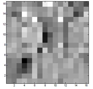
Correlation coefficients of source and target vectors (16th order LSFs) (the darker cell is the lager element)
In Equation (5), the correlation between the source vector x and the target vector y is the term
 . In statistical terms, the correlation coefficients determine the linear association between the two vectors. However, our experiments shows that in many cases the correlation coefficients in this term are very small, meaning that modeling the relationship between x and y by a linear function is inadequate. In our experiments, nearly 90% of the elements have values less than 0.1. Moreover, over 50% of the elements are smaller than 0.01.Due to the small values of this correlation term, the converted vectors, F(x) are usually close to
 . This means that whatever the source vector is, the converted vector is very close to the sum of weighted means of target vectors. As a result, the converted speech seems to be over-smoothed.
3. Nonlinear GMM-based Transformation
3.1. Nonlinear Transformation Function: RBF
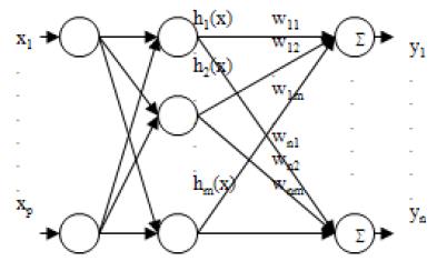
A GMM-based nonlinear transformation has been proposed using Radial Basis Function (RBF) networks by [6], which is a refinement of the Baudoin's model [7]. RBF network is a nonlinear interpolation technique posing the property of best approximation as shown in [8]. Figure 2 shows the structure of a typical three-layer RBF network with p inputs, one hidden layer containing m nodes corresponding to m basis functions, and q outputs. The input vector x = [1,x1,x2,...,xp] is applied to all the basis functions in the hidden layer. The output of each hidden node hi (x), (i = 1, ..., m) is a nonlinear function called a basis or response function. The output of the hidden layer is weighted by a weighted vector wk = [wk0,wk1, ..., wkm]T (note that wk0 is the bias term). Then, the output of the network y = [y1,y2, ..., yq is a weighted sum determined by
where h()x is the (m+1)-dimensional vector and W is a (m + 1) • q weight matrix.
In RBF networks, the choice of basis functions plays an important role in the success of approximation problems. The widely used basis functions include Gaussian functions and spline functions whose parameters are determined empirically as in [7]. In this paper, unlike Baudoin's model, we use a more principled RBF approach presented by [9] in which the basis functions are the normal probability density functions of the GMM of the source speaker. Specifically, we fix the number of basis functions as the number of mixtures of a GMM and then estimate the parameters of the GMM using the EM algorithm. The basis functions then have the form
Note that Equation (7) differs from Equation (2) in the constant term 1/ ((2π)p/2|Σ|1/2) since the basis functions need to be normalized.
The drawback of the RBF method is that it may be difficult to approximate a complex relationship by a global nonlinear function. Therefore, in the next section we propose a refined approach where we approximate the relationship between source and target features by a mixture of locally nonlinear functions, each of which is approximated by an RBF.
3.2. Piecewise RBF
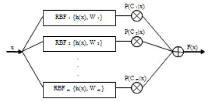
In this section, w e propose a more generalized version of the LSE method where each local linear function is substituted by a local nonlinear function which is modeled by an RBF network. However, since it is hard to determine a different set of basis functions for each local RBF, we use the same set of basis functions h(x) = [1,h1(x,h2(x,...,hm(x) for every local RBF (see Figure 2). Similar to the RBF transformation method above, here the basis function hm(x, (i = 1,...,m) is the “normalized” Gaussian distribution density in Equation (7). Consequently, the transformation function has the following form
The transformation function F( • ) is entirely defined by the p-dimensional vectors νi and the P × p matrices Γi for i = 1,...,m.
These parameters are estimated by linear least squares estimation on the training data so as to minimize the total error
Specially, the least squares optimization of the parameters is the solution of the following set of linear equations
for all t = 1,...,n. In the matrix form, (11) can be written as
Where the two matrix ν and Γ are the unknown parameters of the transformation function. ν is a m × p matrix, Γ is a m2 × p matrix and Y is a n × p matrix containing the target spectral vectors as follows
P is a n × m posterior matrix and Δ is a n × m2 matrix that depends on the conditional probabilities, the source vectors, and the GMM parameters.
The solution for Equation (11) is given by the normal equation
The left most matrix in Equation (13) is symmetric but not positive definite and thus cannot be inverted using the Cholesky decomposition. Therefore, we exploit SVD to compute its pseudo inverse.
4. Experiments
4.1. Experimental Environments
We use the MOCHA-TIMIT speech database [8] to train and evaluate proposed system. For training, 30 sentences were used for each speaker which result in more than 6000 vectors. 10 sentences were used for evaluation. Two male and two female speakers are participated in the experiments. We perform eight conversion tasks, four male-to-female, and four female-to-male conversions. Table 1 show the speaker combination used in our experiments. There are two important distances in voice conversion: the transformation error E(t(n),
 ) and the inter-speaker error E(s(n), t(n) where s(n), t(n,
 denote the source, target, converted speech respectively. All the errors are conceptual and cannot be measured directly. In this experiment, these errors are approximated by objective measures as
where A,B is the two sequences of LSF vectors, n is the number of vectors in each vector sequence, p is the order of LPC and Li,k is the kth component of ith LSF vector.
To take into account the inter-speaker errors, we define the LSF performance index as Equation (15).
The Performance index defined as Equation (15) uses normalized error to compare the performance of different voice conversion tasks across the different speaker combinations. The performance index PLSF is 0 for a simple copy of source speech to the output without conversion. In the case of producing the exact target speech, PLSF is 1. Although ELSF and PLSF are not the standard measures of error between two speech signals, they can be applied to input and output parameters of the conversion system directly. This is the reason why we use them as objective measures.
4.2. Experimental Results
In the experiments, we investigated the influence of the number of mixture components m on the performance of conversion system. LSE and RBF were used as baseline systems and compared with proposed piecewise RBF method. Experiments were performed while increasing m as 1, 2, 5, 8, 16, 32, 64, 128 with fixed LPC order p = 16.
Table 2 shows the experimental results averaged over all speaker combinations. Experimental results show that when the number of mixtures is increased, proposed method gives better results than the baseline systems. This can be interpreted as for the small number of mixtures, linear transformation methods gives better results, however for the large number of mixtures, local non-linear transformation function gives better conversion results by removing the drawbacks of linear and global non-linear transform functions.
5. Conclusions
In this paper, we propose GMM-based piecewise nonlinear transformation methods for voice conversion. Experiments show that the piecewise RBF method is comparable to the linear transformation methods and when the large number of mixtures is used, the proposed method gives a higher accuracy.
Acknowledgments
Implementation of the algorithm in this paper was a collaboration with Mr. Hoang G. Vu and Dr. Jaehyun Bae. Thank to Mr. Hoang G. Vu and Dr. Jaehyun Bae.
References
- S. Moon, “Enhancement of ship’s wheel order recognition system using speaker’s intention predictive parameters”, Journal of Society of Marine Engineering, 32(5), p791-797, (2008).
- S. Nakamura, K. Shikano, and H. Kuwabara, “Voice conversion through vector quantization”, Proceedings of Internaltional Conference on Acoustics, Speech and Signal Processing, p655-658, (1988).
-
Y. Stylianou, O. Cappe, and E. Moulines, “Continuous probabilistic transform for voice conversion”, IEEE Transactions on Speech and Audio Processing, 6(2), (1998).
[https://doi.org/10.1109/89.661472]

-
A. Kain, and M. Macon, “Spectral voice conversion for text-to-speech synthesis”, Proceedings of Internaltional Conference on Acoustics, Speech and Signal Processing, p285-288, (1988).
[https://doi.org/10.1109/ICASSP.1998.674423]

- A. Kain, “High resolution voice transformation”, Ph.D dissertation, Oregon Graduate Institute of Science and Technology, (2001).
- C. Orphanidou, I. Moroz, and S. Roberts, “Wavelet-based Voice morphing”, Journal of World Scientific and Engineering Academy and Society, 10(3), p3297-3302, (2004).
- G. Baudoin, and Y. Stylianou, “On the transformation of speech spectrum for voice conversion”, Proceedings of International Conference on Spoken Language Processing, p1405-1408, (1996).
- C. Bishop, “Neural networks for pattern recognition”, Clarendon Press, Oxford, (1995).
- A. Dempster, N. Laird, and D. Rubin, “Maximum likelihood from incomplete data via the EM algorithm”, Journal of Royal Statistical Society, 39, p1-22, 22-38, (1977).


