Hydrodynamic coefficients of a chain model by using the Morison equation

1. Introduction

The design of mooring lines for floating offshore structures is important to their safety. Environmental influence on the mooring lines, such as waves and current, can lead to fatigue damage on the structures [1]. Thus, a number of scientific studies have focused on the design of mooring lines with regard to their environmental conditions. Even though chains are the most common type of mooring lines for existing structures, most of previous research estimated hydrodynamic coefficients based on circular cylinders.

Many researchers have focused on finding the coefficients for several model types under different flow conditions. Circular cylinder model tests have been carried out under oscillating [2][3] and periodic flows [4]. Some tests were implemented for other types of objects [5][6] and mooring lines made of chain [7].

This study presents the first step in an analysis of mooring lines made of chains. The hydrodynamic forces and moments for three different sizes of twisted link chains and circular cylinders were measured to calculate coefficients in a wind tunnel [8]. Corresponding hydrodynamic coefficients were firstly estimated from the Morison equation and a comparison between chain and cylinder models was also made. In addition, new estimation formulas for chain hydrodynamic coefficients are suggested to complement the Morison equation, which is based on the slender body theory.

2. Wind tunnel measurement

2.1 General

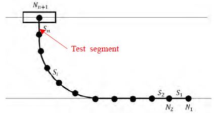
Mooring lines are a combination of several segments, such as chains and wire ropes. Figure 1 shows a discretization of the mooring line into N elements; the top segment under the structure was selected as the test model for this study [9].

Figure 1:

Discretization of mooring line

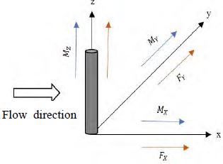
Figure 2 presents a Cartesian coordinate system of the experiment model of the study.

Figure 2:

Cartesian coordinate system

The hydrodynamic coefficients are calculated using a generalized Morison equation, where the added mass and drag coefficients are specified for each element. The Morison equation is a semi-empirical equation for hydrodynamic forces on a slender body in an oscillatory flow. From the equation, hydrodynamic force, F, on a slender body is:

$\[ F=\rho \cdot C_M\cdot V\cdot \frac{dU}{dt}+\frac{1}{2}\cdot \rho \cdot C_X\cdot A\cdot U\left|U\right| \]$

(1)

The Morison equation is the sum of the drag and inertia forces. However, in this test, the rate of velocity change over time, $$ \frac{dU}{dt}$$, is zero because flow velocity is constant. Thus, the coefficients can be calculated as:

(for drag, lift and transverse force coefficient)

$\[ C_{X,Y,Z}=\frac{F_{X,Y,Z}}{\frac{\rho }{2}\cdot U^2\cdot A} \]$

(2)

(for moment coefficient related to vertical axis)

$\[ C_{MZ}=\frac{M_Z}{\frac{\rho }{2}\cdot U^2\cdot l^2\cdot d} \]$

(3)

The forces acting on the cable comprise tension, weight, and external forces. The external force includes fluid-related forces, such as hydrostatic, drag, and inertia forces.

2.2 Experiment conditions

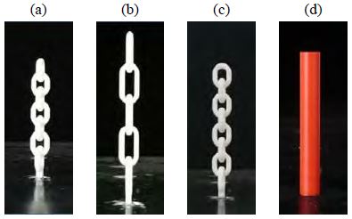
The measurement was carried out with three chain and one circular cylinder models in a wind tunnel. Figure 3 shows four test models. The Reynolds number is applied for the dimensionless calculation of the hydrodynamic coefficients. By definition, the Reynolds number is the ratio of the inertia forces to viscous forces and is formulated as:

$\[ Re=\frac{d\cdot U}{v} \]$

(4)

Figure 3:

Test models: From the left, Chain No.1, Chain No.2, Chain No.3 and Circular cylinder, respectively

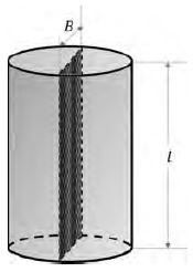
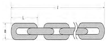
Figure 4 and Figure 5 show definitions of dimensions for the circular cylinder and chain, respectively. The areas of the chain and the circular cylinder should be calculated by using a cross-section of the model.

Figure 4:

Dimension for circular cylinder

Figure 5:

Dimension for chain

Table 1 contains dimension details of the test models and the circular cylinder model has a similar outside width (B: 0.034m) to Chain No.2 (B: 0.032m). The three-dimensional hydrodynamic experiments were carried out under the same conditions as in the model test.

Table 1:

Details of test models

3. Comparison of hydrodynamic coefficients

3.1 Comparison between chain and circular cylinder

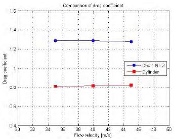
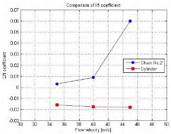
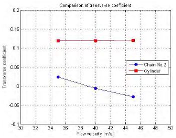
Table 2 and Figure 6 ~ 8 show comparisons of the hydrodynamic coefficients between Chain No. 2 and the circular cylinder. The two models have comparable outside widths and identical experimental conditions, which means every measurement was made under the angle position of 0° at flow velocities of 35 m/s, 40 m/s, and 45 m/s. As shown in Figure 6, the drag coefficient of the chain is larger than that of the cylinder because of its higher roughness. Winkel also shows that such a chain possesses higher drag than a cylinder [10]. However, differences in lift and transverse coefficients are negligible due to the magnitude of the values.

Table 2:

Comparison between Chain No.2 and Cylinder

Figure 6:

Comparison of drag coefficients between Chain No.2 and Cylinder

Figure 7:

Comparison of lift coefficient between Chain No.2 and Cylinder

Figure 8:

Comparison of transverse coefficient between Chain No.2 and Cylinder

3.2 Comparison of three different chains

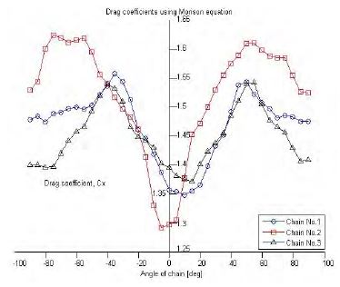
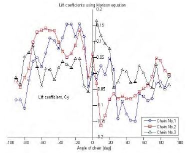
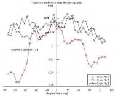
Figure 9 ~ 11 show comparisons between the three chain models. The drag coefficients values are similar for each model, ranging from 1.3 to 1.6. Differences between lift and transverse coefficients are also negligible due to the magnitude of the values.

Figure 9:

Drag coefficients for all chains at Re 0.95 × 105

Figure 10:

Lift coefficients for all chains at Re 0.95 × 105

Figure 11:

Transverse coefficients for all chains at Re 0.95 × 105

4. Estimation formulas for chain models

Owing to the shape characteristic of the chain, it is not suitable to apply the Morison equation directly, which is based on the slender body theory, into the chain models. This section provides newly suggested formulas for the calculation of hydrodynamic coefficients and a comparison between the results of the Morison and suggested equations.

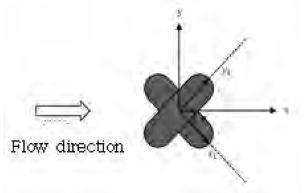
Figure 12 shows a coordinate system and resultant forces on the chain. The value α is an angle between the chain model and the incoming flow.

Figure 12:

Coordinate system and resultant values on chain

The resultant equations of forces and coefficients are based on the Morison equation, considering a rotation angle α and corresponding measured forces, which vary based on the shape of chain to be exposed to the flow.

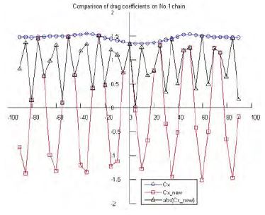
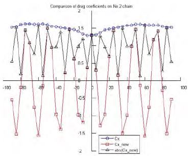
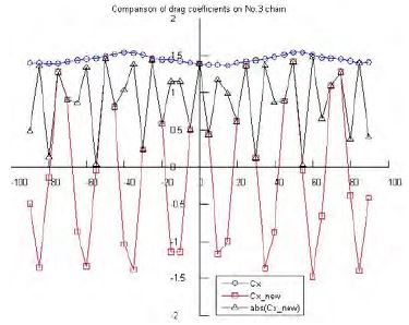
Figure 13 ~ 15 compare drag coefficients of each chain using the Morison equation and newly suggested formula, namely C_X and C_Xnew. The item abs(C_Xnew) is also included to show magnitude of the force, regardless of direction. Maximum drag coefficients values using the new formula are close to the corresponding values using the Morison equation.

Figure 13:

Comparison of drag coefficients for Chain No.1 at Re 0.95 × 105

Figure 14:

Comparison of drag coefficients for Chain No.2 at Re 0.95 × 105

Figure 15:

Comparison of drag coefficients for Chain No.3 at Re 0.95 × 105

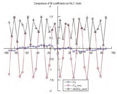
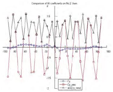
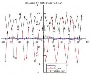
Figure 16 ~ 18 compare lift coefficients of each chain with the Morison equation and the newly suggested formula. On comparison with the drag coefficient results, it can be seen that the lift coefficients using the new formula are greater than the corresponding values using the Morison equation, and the maximum values are close to the respective drag coefficient values. It is conjectured that the lift coefficients are dependent on the flow’s inflow angle, and this is not shown from the Morison equation results.

Figure 16:

Comparison of lift coefficients for Chain No.1 at Re 0.95 × 105

Figure 17:

Comparison of lift coefficients for Chain No.2 at Re 0.95 × 105

Figure 18:

Comparison of lift coefficients for Chain No.3 at Re 0.95 × 105

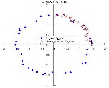
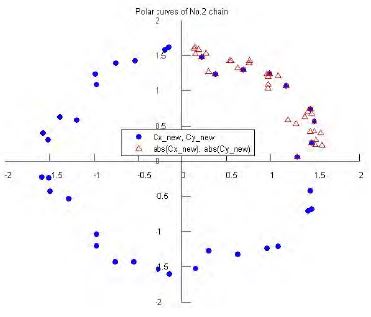
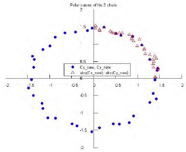
Figure 19 ~ 21 show the polar curves of lift and drag coefficients using Equation (5). Blue points indicate the new formula results and red triangles indicate the absolute values of these results. All of the polar curves are shaped like a pie graph and have almost the same values.

Figure 19:

Polar curve of Chain No.1

Figure 20:

Polar curve of Chain No.2

Figure 21:

Polar curve of Chain No.3

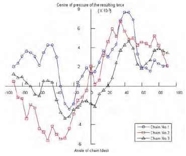
Figure 22 shows the center of pressure of the resulting force from the lift and drag coefficients for the three chains using Equation (6).

Figure 22:

Center of pressure of resulting force

5. Conclusion

There have been many experimental and empirical tests implemented to verify coefficients for a circular cylinder. However, empirical data on Morison force coefficients for a chain-shaped model are scarce. In this study, hydrodynamic force acting on a chain was measured and coefficients were calculated. The tests involved free and forced oscillations of a chain in a wind tunnel.

Firstly, a comparison between the chain and cylinder models showed that higher object roughness causes a higher drag coefficient. The drag coefficient for the chain model was greater than that of the circular cylinder model. Otherwise, lift coefficients for both models were nearly identical. Additionally, the cylinder model had a fixed transverse coefficient, whereas the chain model had a curved-values transverse coefficient.

Secondly, a comparison of the various chain shapes and sizes showed almost the same coefficient values. Transverse coefficients had negligible values, and the chain drag coefficient was approximately 1.5 at a Reynolds number of 0.95 × 10⁵. Generally, the drag coefficient of a circular cylinder is 0.78 at L/D = 8, (L: length of cylinder, D: width of cylinder) with a Reynolds number ≥ 10⁴.

Lastly, a set of new formulas for the hydrodynamic force was suggested and their corresponding coefficients represent characteristics of the chains better than the coefficients from forces calculated by the Morison equation, which is based on circular cylinder models. However, additional verification with various element positions should be carried out in future studies.

This study should be repeated in a water tank and with computational fluid dynamics (CFD), and the results of the present study, water tank, and CFD should be compared to obtain a value close to the actual value in a three-dimensional flow situation.

References

• DNV, Position mooring, DNV-OS-E301, DNV, Norway, (2010).
• J. R. Driscoll Jr., Forces on Cylinder Oscillating in Water, M.S Thesis, Department of Mechanical Engineering, Naval Postgraduate School, United States of America, (1972).
• O. S. Madsen, “Hydrodynamic force on circular cylinder”, Applied Ocean Research, vol. 8(no. 3), p151-155, (1986). [https://doi.org/10.1016/s0141-1187(86)80014-1]
• C. J. Garrison, J. B. Field, and M. D. May, “Drag and inertia forces on a cylinder in periodic flow”, Journal of the Water ways Port, Coastal and Ocean Division, American Society of Civil Engineers, vol. 103(no. 2), p193-204, (1977).
• A. Bliek, Dynamics Analysis of Single Span Cables, Ph.D. Thesis, Department of Ocean Engineering, Massachusetts Institute of Technology, United States of America, (1984).
• L. E. Borgman, “Random hydrodynamic forces on objects”, The Annals of Mathematical Statistics, vol. 38(no. 1), p37-51, (1967). [https://doi.org/10.1214/aoms/1177699057]
• W. S. Yang, Hydrodynamic Analysis of Mooring Lines Based on Optical Tracking Experiments, Ph.D. Dissertation, Department of Ocean Engineering, Texas A&M University, United States of America, (2007).
• S. Schreier, Wind Tunnel Measurement System Bericht, Internal Document, Faculty of Mechanical Engineering and Marine Technology, University of Rostock, Germany, (2015), (in German).
• O. M. Faltinsen, Sea Loads on Ships and Offshore Structures, Cambridge, United Kingdom, Cambridge University Press, (1990).
• H. J. Winkel, “Hydrodaynamic forces at a smooth cable – scrouton spiral”, Contributions on the Theory of Fishing Gears and Related Marine Systems, vol. 3, p251-260, (2003).