[ Original Paper ]

Journal of the Korean Society of Marine Engineering - Vol. 41, No. 5, pp.452-460

ISSN: 2234-7925 (Print) 2234-8352 (Online)

Print publication date 30 Jun 2017

Received 02 May 2017 Revised 01 Jun 2017 Accepted 08 Jun 2017

DOI: https://doi.org/10.5916/jkosme.2017.41.5.452

Forecasting greenhouse gas emissions in the Korean shipping industry using the least squares adjusted with pseudo data

Jeong-Woo Kim¹ ; Joo-Cheol Kim² ; Jeong-Tae Kim³ ; Jae-Hwan Kim^†

1School of Economics, Yonsei University orignkik1@gmail.com
2School of Economics, Yonsei University, Tel: 02-2123-5498 joocheol@yonsei.ac.kr
3Department of Marine Engineering, Korea Marine Engineering University, Tel: 051-410-4884 jt0998@gmail.com

Correspondence to: ^†Department of Data Information, Korea Maritime and Ocean University, 727, Taejong-ro, Yeongdo-gu, Busan 49112, Korea, E-mail: jhkim@kmou.ac.kr, Tel: 051-410-4374

Copyright ⓒ The Korean Society of Marine Engineering
This is an Open Access article distributed under the terms of the Creative Commons Attribution Non-Commercial License (http://creativecommons.org/licenses/by-nc/3.0), which permits unrestricted non-commercial use, distribution, and reproduction in any medium, provided the original work is properly cited.

Abstract

The problem of greenhouse gas emissions is considered as one of the most important problems in global environmental issues. In the shipping industry, the problem of greenhouse gas emissions is also a critical issue, and International Maritime Organization published 3rd report on greenhouse gas in 2014. Studies on greenhouse gas emissions in the shipping industry have mainly focused on policy issues or an estimation of greenhouse gas emissions from fuel consumption. In this paper, we forecast greenhouse gas emissions using nonparametric statistical methods. Among the nonparametric statistical methods, local regression with one-sided kernel function is used to forecast a future value. However, setting a future value as an unknown in the optimization procedure gives the difference between the test error and the training error. We propose the adjusted least squares with pseudo data to reduce this difference and to get a more accurate forecast. Theoretical bases on our method and empirical results are presented comparing the various types of pseudo data.

Keywords:

Greenhouse gas, Local regression, One-sided kernel function, Pseudo-data

1. Introduction

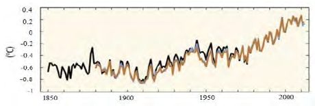
Global warming is the largest part of the climate change problem. According to the IPCC Fifth Assessment Report [1] (see Figure 1 and Figure 2), the global surface temperature increased by about 0.85 degrees Celsius from 1880 to 2012. Since the industrial era, greenhouse gas(GHG) emissions have risen sharply and are believed to be responsible for global warming.

Figure 1:

Land and sea surface temperature difference trend

Figure 2:

GHG emissions trend

In January 2014, “Roadmap For Achieving The National GHG Reduction Target” was announced in Korea. In addition, domestic GHG emissions trading system has been introduced since 2015. Since Korea's GHG reduction target submitted to the UNFCCC was 30% (compared to 1990) by 2020 as in [2], Korea should make efforts to reduce GHG emissions.

According to the International Maritime Organization (IMO) GHG study in 2014 [3], CO₂ emissions from international shipping industry are about 796 million tons. This amount accounts for 2.2% of the world's CO₂ emissions.

Therefore, concern in the GHG emissions in the shipping industry problem has been increasing in related fields. Nadine et al. [4] has done research on how to allocate CO₂ emissions from the shipping industry among countries. They argued that emissions should be allocated according to the nationality of the ship operating company. Crist [5] estimated the level of GHG emissions from international maritime industry and focused on some factors for future emission levels such as GHG-reducing technology options, speed reduction and fuel switching. James et al. [6] predicted that energy consumption would increase as global maritime transport increases, resulting in an increase in future GHG emissions. Choi et al. [7] estimates GHG emissions from domestic shipping industry and fishery using the GHG emissions factor of IPCC Guideline. Lee et al. [8] experimented with a training ship to calculate GHG emissions with fuel consumption for one year. Paik et al. [9] analyzed the domestic shipbuilding industry by process, and predicted the GHG emissions from using ARIMA model. They forecasted that the GHG emissions in 2035 will be more than double from 2007. Kim et al. [10] considered the problem of determining the ship speeds and fleet sizes to reduce GHG emissions and suggested the carbon tax and the emission trading scheme as actual regulations. As above, existing studies on GHG emissions in shipping industry mainly focused on policy issues or estimation of greenhouse gas emissions from fuel consumption in an engineering point of view. In the latter case, IPCC emission factors are used to estimate the GHG emissions. Since the emission factors have not been updated for a long time and the emission amount may vary depending on the type of ship and the operating environment, an estimation of GHG emissions through statistical methods considering the latest situations in Korea can be meaningful. In this study, we carried out GHG emissions forecasting using nonparametric statistical methods. Nonparametric statistics methods are useful when a mean function is not clear and/or a process is very volatile. Among the nonparametric statistical methods, local regression is a representative one.

Local regression studies related to forecasting can be found in the practical areas such as traffic forecasting, energy demand forecasting and weather forecasting. Sun et al. [11] used local linear regression to predict short-term traffic volumes and showed that this method is better than the local constant regression and kNN method. Elattar et al. [12] showed that SVM regression using the regular parameters with the local weight outperforms the result from the standard SVM regression in forecasting an electric load. Pinson et al. [13] used a new type of local regression to forecast a wind power production. In their study, the coefficients are obtained from a Total Least squares (TLS) criterion that uses orthogonally fitted residuals.

When using the kernel function in local regression, we need points on both sides of the target point. However, in the forecasting problem, it is impossible to use the data to the right side of the target point, i.e., future values. This leads us to use one-sided kernel. One of the previous studies dealing with forecasting problem based on one-sided kernel approach is the work of Gijbels et al. [14]. Li et al. [15] also developed the onesided kernel approach for extrapolation in an arbitrarily small region.

To predict future values using the above two techniques, the predicted value is set as an unknown. This is one of the causes of the difference between the test error and the training error. In this study, we implement the adjusted least squares with pseudo data for this unknown, transforming the test error into the training error, and predict a future value.

The remainder of the paper is organized as follows. The adjusted least squares method using local regression and onesided kernel is introduced in Section 2. In Section 3, the empirical results on the forecasting accuracy of the GHG emissions using this method are presented. Conclusions and future works are mentioned in Section 4.

2. Methods

2.1 Local regression

Local constant regression (or kernel regression) was first proposed by Nadaraya [16] and Watson [17] as a way of locally estimating the true value by averaging points when given a certain bandwidth.

An estimator by local constant regression for some y at x using a uniform kernel is as below,

y ̂ = ∑ t = 1 T 1 X t - x ≤ h y t / ∑ t = 1 T 1 X t - x ≤ h

(1)

where 1(•) is the indicator function and h is a bandwidth parameter. Generalizing local constant regression, local polynomial regression was proposed by Cleveland et al. [18]

y ̂ = e 1 T X x T W x X x - 1 X x T W x Y

(2)

where,

X x = 1 x 1 - x ∙ ∙ ∙ x 1 - x p ∙ ∙ ∙ ∙ ∙ ∙ ∙ ∙ ∙ ∙ ∙ ∙ 1 x T - x ∙ ∙ ∙ x T - x p, W x = d i a g 1 ≤ t ≤ T K x t - x h, Y = y 1, ⋯, y T

and e₁ is the column vector of 1 in 1st position and 0’s in other positions, K(•) is a kernel function.

As seen in Equation (1) and (2), without assuming any specific function ahead except for a kernel function, we can estimate a data generating process by using local regression.

2.2 One-sided kernel

In order to make use of kernel function using local regression for the forecasting problem, we need to use the asymmetric kernel function, i.e., one-sided kernel function. Taking a gaussian kernel function as an example,

K u = 1 2 π e x p - u 2 2 1 u ≤ 0

(3)

where u is a standardized variable. To consider only one side of the support, the indicator function is used. One-sided kernel is proposed by Muller [19] to detect the discontinuities in nonparametric regression. The discontinuity usually occurs at the boundaries of an interval and it can cause inconsistency or bias of the estimator, that is, a boundary effect. There are some studies to solve this problem, and as recent studies Campo et al. [20] and Hickman et al. [21] used one-sided kernel function to solve this problem.

Considering that the boundary point is an end point in a given interval, one-sided kernel can be used for the forecasting problem. Gijbels et al. [14] theoretically showed how the exponential weighted moving average (EWMA) is identical with local regression with one-sided kernel function in the forecasting problem. Li et al. [15] also used one-sided kernel method to extrapolate a future value with some modified cross-validations.

2.3 Pseudo data

In nonparametric statistics, pseudo data method is used to solve a boundary effect when estimating a kernel density function. Cowling et al. [22] used pseudo data beyond the support of the density. They made pseudo data from using data points to the one side of a certain point. According to an example in their paper, a pseudo data point X_-1 to the left of the support [0, 1] can derived by X_(-1) = 3X₍₁₎ + X₍₂₎, where X_(i) is the order statistics of the data X_i. Therefore, the pseudo data can be some data points beyond the support, but not include a boundary point that should be a forecast in the forecasting problem.

As another way to generate pseudo data, the reflection data method is also suggested by Cline et al. [23]. As long as the derivative of the density is zero at the boundary of the support, this method just adds {-X₁, -X₂, . . . , -X_n} to the other side of original data set {X₁, X₂, . . . , X_n}. This method is basically based on the symmetry of the density function, which makes it possible to obtain pseudo data set on the other side of the given support.

Unlike the density estimation using the pseudo data idea, in the forecasting problem we cannot expect a symmetry feature helpful for making pseudo data. Instead, candidates for pseudo data in the forecasting problem can be a value at the current point, a sample mean up to the current point or a predicted value by linear regression. We use these three types of pseudo data in this study.

2.4 Least squares adjusted with pseudo data

Consider a model,

y t = m x t + e t

(4)

where x_t is a predictor and y_t is a response variable via a mean function m(_xt), and e_t is an independent and identically distributed random variable with zero mean and unit variance and is independent of the x_t.

In the forecasting problem using local regression, the goal is to minimize test error or prediction error (PE),

P E m ̂ = E y T + 1 - m ̂ x T + 1; h 2 | T

(5)

where Τ = {(x_t, y_t) : t = 1, ..., T}.

For a mathematical convenience, the expected prediction error(EPE) is be more useful,

E P E m ̂ = E y T + 1 - m ̂ x T + 1; h 2

(6)

With a discrete data set, Equation (6) is approximated by the average squared residuals(ASR) or a training error,

A S R h = T - 1 ∑ t = 1 T y t - m ̂ x t; h 2

(7)

Denote the minimizer of (7) as $h ̂ o$

h ̂ 0 = arg ⁡ l i m h ≥ 0 A S R h

(8)

Using $h ̂ o$ , we obtain the local constant estimator $y ̂ T + 1$

y ̂ T + 1 = ∑ t = 1 T K x t - x T + 1 h ̂ 0 y t / ∑ t = 1 T K x t - x T + 1 h ̂ 0

(9)

This is the basic scheme of the forecast using one-sided kernel used in the previous studies, such as [14][15]. However, instead of approximating as Equation (7), if we can transform the test error minimization problem into the training error minimization problem we can expect a less test error than before. To do this, of course, we need to know the actual value in the future, but it is impossible. Instead, we propose pseudo data $y ̃ T + 1$ in substitution for actual y_T+1 to obtain a pseudo-training error as Equation (10), from which the pseudo-optimal bandwidth for forecasting y_T+1 is obtained. As mentioned in 2.3, we use three types of pseudo data for $y ̃ T + 1$ .

With $y ̃ T + 1$ , we can construct a new set, Τ_p = Τ ∪ {(x_T+1, $y ̃ T + 1$ )}. To express training error using pseudo data, denote the pseudo-training error by PTE,

P T E m ̂ = E y T + 1 - m ̂ x T + 1; h 2 | T p

(10)

Then, pseudo ASR including $y ̃ T + 1$ becomes

A S R h = T + 1 - 1 ∑ t = 1 T y t - m ̂ x t; h 2 + y ̃ T + 1 - m ̂ x T + 1; h 2

(11)

Denote the minimizer as $h ̂ p$

h ̂ p = arg ⁡ l i m h ≥ 0 A S R h

(12)

Recall that PE = MSE + $σ e 2$ , where MSE is a mean square error and MSE=Bias² + Var. Using the standard result of kernel density estimation

V a r m ̂ x T + 1; h x 1, …, x T + 1 ≤ V a r m ̂ x T + 1; h x 1, …, x T

(13)

is derived as in [14][24].

Then, we obtain

E y T + 1 - m ̂ x T + 1; h 2 | T p ≤ E y T + 1 - m ̂ x T + 1; h 2 | T

(14)

Among the types of pseudo data used in this study, a sample mean would outperform a current value at T. Unless a given process follows a martingale process E(y_{T +1}| Τ) = y_T , it would be better to approximate y_{T +1} by E(y_t| Τ) rather than y_T. That is,

E E y T + 1 - E y t T ≤ E E y T + 1 - y T |

(15)

One can also find a study as [25] that shows the forecast by a sample mean can be as accurate as the forecast of the other methods.

3. Empirical Results

The data set in this study is summarized in the Table 1. The oil data are collected from Petronet [26] and domestic GHGs are obtained from KGWAC [27].

Table 1:

Descriptive statistics(Unit : bbl, ppm)

The number of months used is 50 from Nov. 2011 to Dec. 2015 for four types of data. The period of the forecasting GHGs is from May. 2014 to Dec. 2015, and each forecast uses the data up to the current point.

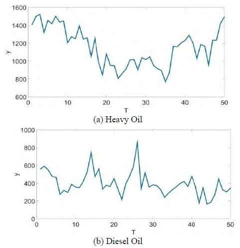
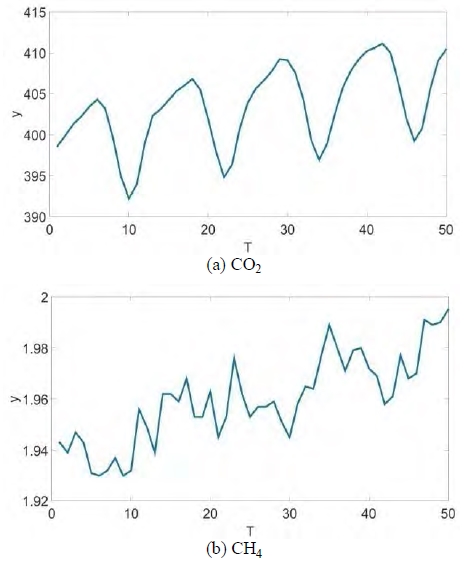
Heavy oil is the main fuel in the marine transportation industry in our country, and diesel oil is mainly used in the offshore fisheries [28]. Among the six GHGs, CO₂ is the largest emission gas by about 77% and CH₄ is the second largest emission gas by about 14% [29].

The trend of each data is as below. Since diesel oil is the main fuel in the domestic fishing industry, its trend is more stable than the heavy oil trend affected by the global economy. The trend of CO₂ emission shows a more periodic feature than the trend of CH₄ due to a seasonal effect, however both show increasing trends.

Figure 3:

Monthly Usage

Figure 4:

Monthly emissions

We carry out four empirical tests; using heavy oil as the predictor for CO₂ and CH₄, and diesel oil as the predictor for CO₂ and CH₄. We apply both local constant regression and local linear regression to each forecasting. An exponential kernel function is used for every forecasting as in [14], and all the values used are standardized.

We use three types of pseudo data, a value at the current point(PSEUDOT), a sample mean up to the current point(PSEUDOm) and a predicted value by linear regression(PSEUDOl), and results from using these pseudo data are compare to the result of EWMA used in [14]. We denote it by Actual when the actual future data at T+1 is assumed to be known, and calculated by ordinary EWMA.

3.1 Case I: CO₂ and CH₄ by Heavy Oil

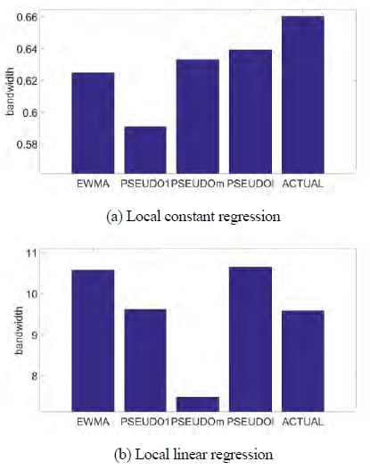
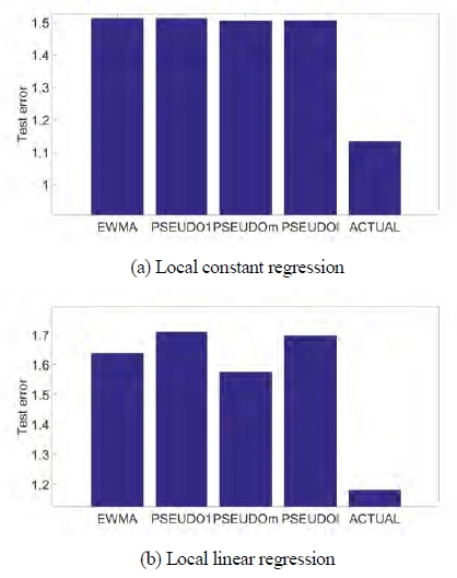
Table 2 and 3 show the comparison of forecasting accuracy across the different methods when heavy oil is used as the predictor for CO₂.

Table 2:

Comparison of test error and bandwidth (CO2 by heavy oil): Local constant regression

Table 3:

Comparison of test error and bandwidth (CO2 by heavy oil): Local linear regression

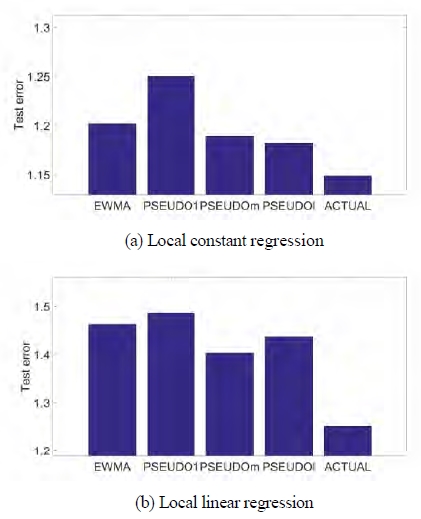
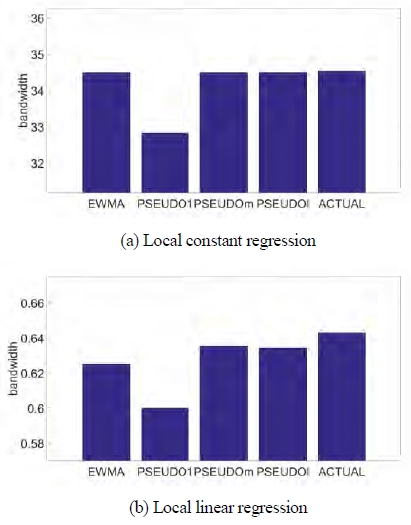
When using local constant regression for CO₂ case, the test error of PSEUDOl is smallest and PSEUDOm is second smallest, which is also less than the test error of ordinary EWMA used in [14]. The test error of Actual is a lower bound by assuming that we can know the value at T+1. The bandwidth of PSEUDOl is larger than the bandwidth of PSEUDOm. Intuitively, the larger bandwidth is used, the more representative value we can expect when forecasting a future value. In the following tables we can also see that bandwidths of proposed methods are mainly larger than that of EWMA, which is advantageous of reducing a variance in test error.

Figure 5:

Test error of CO2 by heavy oil

Figure 6:

Bandwith of CO2 by heavy oil

In the local linear regression case, test error of PSEUDOm is smallest and PSEUDOl is second smallest. PSEUDOT does not show any better result in both cases. Note that the test errors from local constant regression are less than those from local linear regression, and this result is also found in the following cases, which implies that the relationship between the predictor and the response is not a definite linearity.

of forecasting accuracy when CH₄ is forecasted by heavy oil. Unlike the previous result, PSEUDOm outperforms other methods both in local constant regression and in local linear regression. PSEUDOl outperforms EWMA in local constant regression, however it cannot in local linear regression.

Bandwidth of PSEUDOm is second largest in local constant regression and largest in local linear regression.

Table 4:

Comparison of test error and bandwidth (CH4 by heavy oil): Local constant regression

Table 5:

Comparison of test error and bandwidth (CH4 by heavy oil): Local linear regression

Figure 7:

Test error of CH4 by heavy oil

Figure 8:

Bandwidth of CH4 by heavy oil

3.2 Case II: CO₂ and CH₄ by Diesel Oil

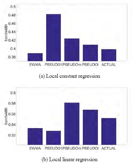
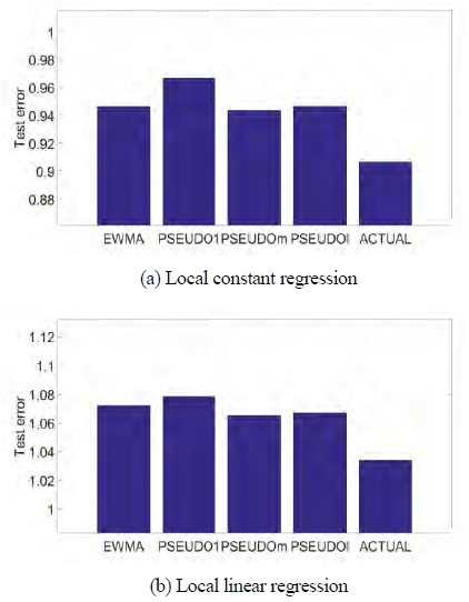
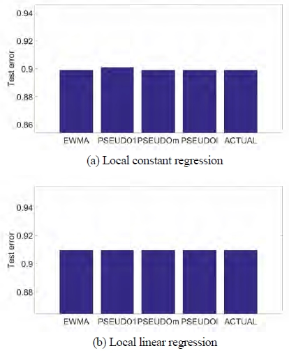
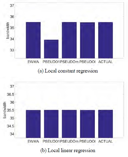
CO₂ and CH₄ gas emissions are forecasted using the usage of diesel oil. For CO₂ case, the results are shown in Table 6 and 7. PSEUDOm shows less test error than EWMA, PSEUDOT and PSEUDOl as before. PSEUDOl also shows a good performance as previous cases. However, the results of test error are mainly smaller than the heavy oil case. This may be due to the fact that diesel oil is a main fuel for the offshore fisheries, which is more related to the domestic GHGs. Bandwidths across the methods are similar to one another except for PSEUDOT, which is also related to the small differences of test error over the methods.

Table 6:

Comparison of test error and bandwidth (CO2 by diesel oil): Local constant regression

Table 7:

Comparison of test error and bandwidth (CO2 by diesel oil): Local linear regression

Figure 9:

Test error of CO2 by diesel oil

Figure 10:

Bandwidth of CO2 by diesel oil

Table 8 and 9 show the result on the CH₄ emissions by diesel oil. Unlike the previous cases, we cannot see any distinct test error difference across the methods including even Actual. From this, we may be able to expect that diesel oil is not an important factor for CH₄ gas emission. Based on it, the test errors from local constant regression are quite similar to those from local linear regression. Similar to the result of test error, bandwidths are also similar across the methods.

Table 8:

Comparison of test error and bandwidth (CH4 by diesel oil): Local constant regression

Table 9:

Comparison of test error and bandwidth (CH4 by diesel oil): Local linear regression

Figure 11:

Test error of CH4 by diesel oil

Figure 12:

Bandwidth of CH4 by diesel oil

4. Conclusions

Greenhouse gas emissions problem is one of the most important factors to global warming. The problem of greenhouse gas emissions in the shipping industry has become a critical issue. With the increasing concern for GHG emissions policy studies or studies on estimation of greenhouse gas emissions studies have been mainly carried out in the related fields.

In this paper, we used nonparametric statistical methods to forecast greenhouse gas emissions. Based on local regression with one-sided kernel function, we proposed the adjusted least squares with pseudo data to obtain a more accurate forecast. It offers a better forecasting accuracy with simply adding pseudo data to an original dataset, and can be easily applied to other optimization tool by its simplicity.

The idea on the adjusted least squares with pseudo data is inspired from the use of pseudo data in the kernel density estimation [22][23]. We tested the performance of three pseudo data, the current point before a forecast, a sample mean up to the current point and an estimate by linear regression.

Using heavy oil and diesel oil as predictors, we forecast CO₂ and CH₄ gas emissions. As a result, the method with a sample mean as a pseudo data point showed better forecasting accuracy than EWMA and other pseudo data methods. The pseudo data method using an estimate by linear regression gives good performance depending on a data set.

However, the degree of the forecasting accuracy improvement by the adjusted least squares with pseudo data can be weak as the size of a sample is very large. In the future work, this part can be addressed for applying this method to a very large sample by using ideas from kNN, local prediction [12], etc.

References

The Core Writing Team (IPCC), Rajendra K. Pachauri, and Leo Meyer, AR5: Fifth Assessment Report, Intergovernmental Panel on Climate Change (IPCC), (2014).
S. Y. Lee, K. M. Kim, and Y. J Kim, A study on the status of greenhouse gas mitigation policy instruments and its improvement(2) - Focusing on Realization of the National Greenhouse Gas Reduction Roadmap, Korea Environment Institute, (2014), (in Korean).
T. W. P. Smith, J. P. Jalkanen, B. A. Anderson, J. J. Corbett, J. Faber, S. Hanayama, E. O'Keeffe, S. Parker, L. Johansson, L. Aldous, C. Raucci, M. Traut, S. Ettinger, D. Nelissen, D. S. Lee, S. Ng, A. Agrawal, J. J. Winebrake, M. Hoen, S. Chesworth, and A. Pandey, Third IMO GHG Study 2014, International Maritime Organization (IMO), (2014).
N. Heitmann, and S. Khalilian, “Accounting for carbon dioxide emissions from international shipping: Burden sharing under different UNFCCC allocation options and regime scenariosm”, Marine Policy, 35(5), p682-691, (2011). [https://doi.org/10.1016/j.marpol.2011.02.009]
P. Crist, Greenhouse gas emissions reduction potential from international shipping, OECD/ITF Joint Transport Research Centre Discussion Paper, (2009).
J. J. CORBETT, C. Wang, J. J. Winebrake, and E. Green, Allocation and forecasting of global ship emissions. Clean Air Task Force Report, (2007).
S. J. Choi, S. K. Park, Y. K. Jang, H. K. Lee, E. H. Hwang, and C.K. Bong, “A study on the greenhouse gas emissions from ships in Korea”, Journal of Korean Society of Transportation, 28(6), p33-42, (2010), (in Korean).
S. D. Lee, D. K. Koh, and S. H. Jung, “A study on the greenhouse gas emission from ships with training ship HANBADA”, Journal of the Korean Society of Marine Engineering, 38(3), p240-245, (2014), (in Korean). [https://doi.org/10.5916/jkosme.2014.38.3.240]
C. H. Paik, H. G. Kim, Y. J. Kim, and Y. J. Chung, “A bottom-up approach for greenhouse gas Emission analysis of Korean ship building industry”, Korean Management Science Review, 31(1), p41-48, (2014), (in Korean). [https://doi.org/10.7737/kmsr.2014.31.1.041]
H. J. Kim, and J. K. Kim, “Model for determining ship speed and number of ships considering greenhouse gas emission regulations”, Proceedings of the Autumn Conference of Korean Institute of Industrial Engineers, p494-499, (2011), (in Korean).
H. Sun, H. X. Liu, H. Xiao, R. R. He, and B. Ran, “Short term traffic forecasting using the local linear regression model,” In 82nd Annual Meeting of the Transportation Research Board, Washington, DC, (2003).
E. E. Elattar, J. Y. Goulermas, and Q. H. Wu, “Electric load forecasting based on locally weighted support vector regression”, IEEE Transactions on Systems, Man, and Cybernetics, Part C, 40(4), p438-447, (2010). [https://doi.org/10.1109/tsmcc.2010.2040176]
P. Pinson, H. A. Nielsen, H. Madsen, and T. S. Nielsen, “Local linear regression with adaptive orthogonal fitting for the wind power application”, Statistics and Computing, 18(1), p59-71, (2008). [https://doi.org/10.1007/s11222-007-9038-7]
I. Gijbels, A. Pope, and M. P. Wand, “Understanding exponential smoothing via kernel regression”, Journal of the Royal Statistical Society: Series B (Statistical Methodology), 61(1), p39-50, (1999). [https://doi.org/10.1111/1467-9868.00161]
X. Li, and N. E. Heckman, “Local linear extrapolation”, Journal of Nonparametric Statistics, 15(4-5), p565-578, (2003). [https://doi.org/10.1080/10485250310001605432]
E. A. Nadaraya, “On estimating regression”, Theory of Probability & Its Applications, 9(1), p141-142, (1964).
G. S. Watson, “Smooth regression analysis”, Sankhy: The Indian Journal of Statistics, Series A, 26(4), p359-372, (1964).
W. S. Cleveland, and S. J. Devlin, “Locally weighted regression: an approach to regression analysis by local fitting”, Journal of the American Statistical Association, 83(403), p596-610, (1988). [https://doi.org/10.2307/2289282]
H. G. Muller, “Change-points in nonparametric regression analysis”, The Annals of Statistics, 20(2), p737-761, (1992). [https://doi.org/10.1214/aos/1176348654]
S. Campo, E. Guerre, I. Perrigne, and Q. Vuong, “Semiparametric estimation of first-price auctions with risk-averse bidders”, The Review of Economic Studies, 78(1), p112-147, (2011). [https://doi.org/10.1093/restud/rdq001]
B. R. Hickman, and T. P. Hubbard, “Replacing sample trimming with boundary correction in nonparametric estimation of first-price auctions”, Journal of Applied Econometrics, 30(5), p739-762, (2015). [https://doi.org/10.1002/jae.2385]
A. Cowling, and P. Hall, “On pseudo data methods for removing boundary effects in kernel density estimation”, Journal of the Royal Statistical Society. Series B (Methodological), 58(3), p551-563, (1996).
D. B. H. Cline, and J. D. Hart, “Kernel estimation of densities with discontinuities or discontinuous derivatives”, Statistics: A Journal of Theoretical and Applied Statistics, 22(1), p69-84, (1991). [https://doi.org/10.1080/02331889108802286]
J. W. Kim, and J. C. Kim, “Nonparametric forecasting with one-sided kernel adopting pseudo one step ahead data”, Proceedings of the Autumn Conference of the Korean Data and Information Science Society, p9, (2016).
V. Wieland, and M. H. Wolters, “The diversity of forecasts from macroeconomic models of the us economy”, Economic Theory, 47(2-3), p247-292, (2011). [https://doi.org/10.1007/s00199-010-0549-7]
Petronet, http://www.petronet.co.kr/v3/eng/index.jsp Accessed March 6, 2017.
Korea Global Atmosphere Watch Center, http://www.climate.go.kr/home/Eng/htmls/kgawc/sub1.html Accessed March 6, 2017.
Korea Energy Economics Institute, 2014 Energy Consumption Survey, Ministry of Trade Industry & Energy, (2015), (in Korean).
Encyclopedia of Korean Culture, http://terms.naver.com/entry.nhn?docId=2457048&cid=46637&categoryId=46637 Accessed March 6, 2017 (in Korean).

Data	Months	Mean	Std.Dev.	Max	Min
Heavy Oil	50	1155.6	212.9	771	1523
Diesel Oil	50	397.1	132.3	166	853
CO₂	50	403.3	4.8	392.2	411.1
CH₄	50	2.0	0.02	1.9	2.0

	EWMA	PSEUDOT	PSEUDOm	PSEUDOl	Actual
σ: Standard deviation of bandwidth
Test error	1.2017	1.2497	1.1891	1.1817	1.1488
Bandwidth	0.6249	0.5910	0.6329	0.6394	0.6602
σ	0.3421	0.3408	0.3387	0.3501	0.3475

	EWMA	PSEUDOT	PSEUDOm	PSEUDOl	Actual
Test error	1.4628	1.4864	1.4033	1.4373	1.2504
Bandwidth	10.5716	9.6123	7.4708	10.6452	9.5795
σ	12.7495	12.3675	10.6228	12.6938	12.2322

	EWMA	PSEUDOT	PSEUDOm	PSEUDOl	Actual
Test error	1.5110	1.5112	1.5032	1.5038	1.1325
Bandwidth	0.3885	0.4822	0.4238	0.4091	0.3982
σ	0.1656	0.5759	0.1688	0.1434	0.1628

	EWMA	PSEUDOT	PSEUDOm	PSEUDOl	Actual
Test error	1.6364	1.7085	1.5744	1.6960	1.1800
Bandwidth	0.5332	0.5280	0.5809	0.5678	0.5518
σ	0.3216	0.4518	0.3567	0.3254	0.3399