A study on fault diagnosis technique for rotor sail tilting mechanism using simulation-based data and transfer learning

1. Introduction

With the strengthening of environmental regulations by the International Maritime Organization (IMO), technology development to improve ship energy efficiency and reduce carbon emissions is accelerating worldwide. In particular, as the Energy Efficiency Existing Ship Index (EEXI) and Carbon Intensity Indicator (CII) regulations have come into effect, Rotor Sail systems, which use wind power to assist ship propulsion, are attracting attention as an effective eco-friendly solution. Based on the Magnus Effect, Rotor Sails have the advantage of significantly reducing fuel consumption; however, they involve large rotating structures installed on the deck, which are continuously exposed to harsh marine environments such as high salinity, humidity, and severe vibration. These environmental factors accelerate corrosion and fatigue failure of equipment, serving as a primary cause of reduced system reliability.

Since failures during operation are difficult to maintain immediately and can lead to massive losses such as disruptions in ship schedules or safety accidents, the importance of technology for ensuring the durability of core equipment and preemptively detecting failure signs is being emphasized more than ever [1][2][3].

Traditional ship maintenance has relied on Preventive Maintenance (PM), where parts are replaced according to cycles recommended by manufacturers. However, this has limitations, such as increasing maintenance costs by performing unnecessary replacements even when parts have remaining useful life, or failing to respond to sudden failures that occur between maintenance cycles. Accordingly, a paradigm shift is recently taking place toward Condition-Based Maintenance (CBM) and Prognostics and Health Management (PHM) systems that monitor the real-time status of equipment based on sensor data and predict failure timing. In particular, with the spread of the Fourth Industrial Revolution technologies, fault diagnosis research using deep learning is being actively conducted. This is establishing itself as a core technology for CBM as it can automatically extract fault features from complex mechanical signals and classify states with high accuracy [4].

However, to apply deep learning-based fault diagnosis models to actual industrial sites, especially to newly developed equipment like Rotor Sails, the fundamental problem of "data absence" must be resolved. For the training of deep learning models, data on various failure situations as well as normal data are essential. However, due to the nature of the maritime industry, which prioritizes safety, parts are replaced preemptively before failure occurs, making it extremely difficult to obtain actual failure data. This leads to a class imbalance problem where normal data is abundant but failure data is extremely scarce. In the case of new technologies with short operational histories like Rotor Sails, situations where no failure data is available for training are frequent. This lack of data acts as a major barrier, degrading the performance of existing supervised learning-based artificial intelligence models and hindering field application. To overcome this, data augmentation techniques using Generative Adversarial Networks (GAN) are being studied, but these have limitations in that they only mimic the statistical distribution of data and do not fully reflect the physical failure mechanisms of mechanical systems.

Therefore, this study proposes a hybrid fault diagnosis methodology that generates failure data through physical modeling-based simulations and utilizes it for deep learning model training in environments where obtaining actual failure data is difficult [5]. First, through Failure Mode and Effects Analysis (FMEA), a system reliability analysis technique, core components with the highest failure risk in the Rotor Sail system were identified and selected as diagnostic targets. Subsequently, a physical model was constructed using MATLAB Simulink for the selected components, and virtual failure data was generated by simulating possible failure modes such as leakage and friction. Finally, the generated time-series data was converted into Scalogram images containing time-frequency characteristics, and a diagnostic model was established by transfer learning these into GoogLeNet, a pre-trained Convolutional Neural Network (CNN) model. Through this series of processes, this study aims to demonstrate that a high-reliability fault diagnosis system can be established even for early-stage marine equipment where actual data is insufficient [6].

2. Selection of Target System and FMEA Analysis

2.1 Technology Classification and Configuration of Rotor Sail System

The Rotor Sail system, which is the subject of this study, consists of a rotating body that utilizes the Magnus effect to maximize ship propulsion efficiency and a complex mechanical device that controls and supports it. For the reliability analysis of the system, the overall structure of the Rotor Sail was classified into the following four core subsystems based on their functional characteristics.

The Outer Body Structure is a rotating component on the exterior of the Rotor Sail body, composed of composite materials, adhesives, and bolts. Due to limited mold sizes during manufacturing, it consists of two or three parts joined through bonding. These bonded joints are further secured with bolts for enhanced durability. The Inner Steel Structure is divided into four major parts: the Connection Structure, which links the Outer Body Structure to the bearings of the Inner Steel Structure; the Drive System, consisting of a motor, frequency converter, safety switch, and brake resistor to rotate the Outer Body Structure; the Lower Wheels, which utilize bearings to enable rotation; and the Support Steel Tower, which includes ladders and cable racks for internal maintenance. The Tilting Structure serves as the support unit for the Rotor Sail, performing tilting operations to facilitate cargo transport during berthing. It comprises a Hydraulic Unit (the oil supply system for tilting), a Cylinder (the hydraulic structure performing the tilting action), and a Tilting Structure Part that supports the Rotor Sail. The Control System consists of sensors to detect wind speed and direction, along with hardware and software to control the overall system operation.

Table 1:

Technology Classification of the Rotor Sail System

2.2 FMEA Analysis Methodology

To identify critical failure components, Failure Mode and Effects Analysis (FMEA) was performed in accordance with the international standard IEC 60812. The targets of the analysis included the four systems and sub-components previously classified, and potential failure modes for each part were identified. For risk assessment, the criteria from the QS9000 standard were simplified, classifying Severity (S), Occurrence (O), and Detection (D) into 5, 3, and 4 levels, respectively. The specific evaluation criteria for each factor are summarized in Table 2.

Table 2:

Evaluation criteria for Severity, Occurrence, and Detection rankings

These factors were evaluated on their respective scales by an expert committee comprising three industry and academic specialists, each with over 20 years of experience in the relevant field. The priority of failures was determined by calculating the Risk Priority Number (Equation (1)), which is the product of these three factors [7].

$\[ RPN=\mathrm{ }\mathrm{S}\times \mathrm{O}\times \mathrm{D} \]$

(1)

2.3 Selection of Core Equipment Based on FMEA

FMEA was conducted for a total of 321 failure modes, and Figure 1 below shows the results of analyzing the average RPN values for each system.

Figure 1:

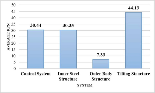
Average RPN Values by the Rotor Sail System

The Tilting Structure exhibited the highest risk level, with an RPN of 44.13. This figure is significantly higher than those of the Inner Steel Structure (30.35) and the Control System (30.44), and it represents a vastly higher risk level compared to the Outer Body Structure (7.33). Because a failure in the Tilting Structure can lead to catastrophic accidents such as the overturning of the Rotor Sail, it received a high average score of 4.13 (based on a 5-point scale conversion) in the Severity category. Additionally, the Detection score was analyzed to be high due to the absence of a dedicated monitoring system.

To mathematically verify that this system-level averaging process does not mask or dilute critical, high-severity individual failure modes, a linear regression analysis was performed across all 321 identified failure modes. By mapping the individual RPN values against the average RPNs of their respective subsystems, the analysis revealed a strong positive linear correlation with a high coefficient of determination (R² = 0.8118). This high R² value rigorously demonstrates that 81.18% of the total variance in individual risks is explicitly explained by the subsystem-level averages. This empirical distribution proves that subsystems with higher average RPNs consistently encompass the high-risk individual failure modes, confirming the statistical reliability of the prioritization framework without risk dilution.

Figure 2 below shows the results of the RPN analysis by component. The hydraulic cylinder (Cylinder), a key driving component of the Tilting Structure, recorded the highest risk level among all parts with an average RPN of 62.4. This was followed by the Lower Wheels (48.0), which are bearing components. As a core power transmission device for tilting operations, failures in the hydraulic cylinder—such as leakage, friction, and fatigue failure—cause a total loss of functionality for the entire system.

Figure 2:

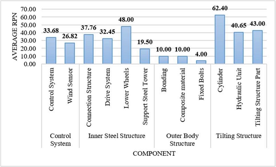
Average RPN Values by the Rotor Sail Component

Therefore, this study selected the hydraulic cylinder of the Tilting Structure, which showed the highest failure risk based on quantitative analysis, as the primary target for developing a fault diagnosis model. Through this, we intend to generate failure data by reflecting major failure modes that occur in actual operating environments—specifically leakage and friction defects—into the simulation model and subsequently verify the diagnostic algorithm.

3. Simulation Modeling for Fault Diagnosis

3.1 Development of MATLAB/Simulink Model

To simulate the dynamic behavior of the hydraulic cylinder, a physical model of the tilting system was constructed using MATLAB Simulink. Figure 3 shows the physical model of the tilting system.

Figure 3:

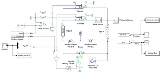
Physical Modeling of the Tilting System

The model consists of two cylinders, flow sensors, and pressure sensors, and was implemented at a 1/10 scale reflecting actual system specifications (piston diameter, stroke, etc.). Additionally, flow and pressure sensors were installed at the cylinder inlets, and the system was modeled to enable the measurement of flow rate and pressure.

3.2 Definition of Failure Modes and Data Generation

The primary failure types occurring in hydraulic cylinders are defined as 'Leakage' resulting from wear between the piston head and the cylinder inner wall, and increased 'Friction' due to poor lubrication. The dynamic behavior according to the variation of each failure factor was simulated through a Simulink-based physical model. Table 3 shows the items and the quantity of the failure data.

Table 3:

Definition of Fault Modes

To ensure the reliability of failure data generation, a simulation-based sensitivity analysis was conducted to quantify the exact parameter threshold ranges. In this study, the engineering threshold for a system fault was defined as the point where the hydraulic flow rate error deviates by 10% or more compared to the normal operational baseline. Accordingly, by isolating the parameter boundaries that induce this 10% performance degradation, the gap for leakage failure was set between 1.001×10^-5 and 2×10^-5m. For friction failure, the breakaway friction ratio was set from 5.6 to 6.5, and the Coulomb friction coefficient was set within the range of 7.1×10^-5 to 5.1×10^-4. Based on these settings, a total of eight state classes were defined, including the normal state, single faults (leakage, breakaway friction, and Coulomb friction), and combined faults consisting of their combinations. By performing more than 200 repeated simulations for each class while randomly varying the parameters, a total of 1,710 time-series datasets for flow rate and pressure were obtained.

4. Deep Learning-based Fault Diagnosis Technique

4.1 Data Pre-processing (Scalogram Transformation)

The flow rate data of the hydraulic cylinder acquired through MATLAB Simulink simulation is in the form of a one-dimensional (1D) time series. In this study, to utilize a CNN model with proven image-based classification performance, a pre-processing step was performed to convert the 1D signal into a 2D image containing both time and frequency characteristics. Continuous Wavelet Transform (CWT) was applied as the transformation technique. Unlike the conventional Fourier Transform, CWT can analyze frequency components while preserving temporal information, making it advantageous for capturing transitional characteristics of abnormal signals such as the timing of failure occurrence. Furthermore, CWT is a technique that analyzes signals in the time domain through correlation with a wavelet function φ having various scales and positions. The CWT equation for a specific signal f(t) is defined as follows:

$\[ W(a,b)=\frac{1}{\sqrt{\left|a\right|}}{\int }_{-\infty }^{\infty }f\left(t\right){\phi }^{\text{*}}\left(\frac{t-b}{a}\right)dt \]$

(2)

Where a is the scale parameter inversely proportional to frequency, and b is the translation parameter that shifts along the time axis. φ^* denotes the complex conjugate of the mother wavelet function φ. Unlike the traditional Short-Time Fourier Transform (STFT), which has limitations in resolution due to a fixed window size, this technique provides a wide time resolution in the low-frequency band and detailed temporal analysis in the high-frequency band, enabling precise capture of minute signal fluctuations occurring during failures. The Scalogram is the result of visualizing the energy density by squaring the absolute value of the coefficients W(a, b) derived from the CWT operation. In this study, the sampling frequency (F_S) was set to 1,000 Hz, and time-series signals with 10,001 data points were converted into Scalogram images.

The Scalogram represents the energy of the signal as color intensity along the time and frequency axes. In this study, 1,710 time-series datasets generated for a total of 8 classes (Case 01–08) were all converted into RGB images with a pixel size of244×244, establishing a dataset that allows the deep learning model to learn the unique visual features of each failure mode. Figure 4 below shows the Scalogram image for a leakage failure.

Figure 4:

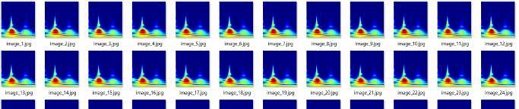
Scalogram Image of Leakage Fault

The collected images were loaded using MATLAB's imageDatastore function, with subfolder names designated as labels. Subsequently, to prevent potential data leakage and eliminate temporal correlation, the entire dataset was randomly partitioned at the discrete image file level using the splitEachLabel function into training data (70%, 1,197 images), validation data (15%, 258 images), and test data (15%, 255 images).

In this process, the training data is used directly for network training, while the validation data is utilized to monitor the training progress at each epoch and ensure the proper convergence of the model's loss and learning rate. Conversely, the test data is strictly excluded from the training and validation phases to ensure an objective calculation of the final model's accuracy.

Although MATLAB's Deep Network Designer automatically normalizes images during training without additional functions, the independently inputted test data underwent a separate normalization process using the augmentedImageDatastore function to match the required input size of the network.

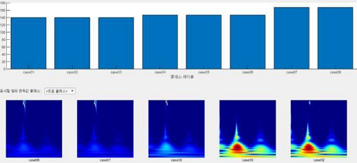
Figure 5 illustrates the detailed composition of the training data, which consists of a total of 1,197 images.

Figure 5:

Training data information

The bar chart at the top shows the quantity distribution for the eight classes (Case 1–8), and the photographs at the bottom present sample images for each case.

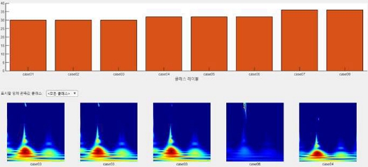
Figure 6 illustrates the detailed composition of the validation data, which consists of a total of 258 images.

Figure 6:

Validation data information

4.2 Construction of Transfer Learning Model (GoogLeNet)

In this study, GoogLeNet proposed by Szegedy et al. [8] was adopted as the classification algorithm for fault diagnosis.

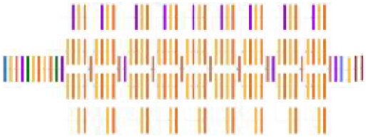
GoogLeNet is a deep neural network (DNN) model that proved its performance by winning the ImageNet Large-Scale Visual Recognition Challenge (ILSVRC) 2014 [8]. Despite having a structure of 22 deep layers, this model is characterized by achieving higher classification accuracy with significantly fewer parameters—approximately 1/12th—compared to its predecessor, AlexNet. The Inception module, the core structure of GoogLeNet, effectively extracts image features by performing convolution and pooling operations with various kernel sizes in parallel. Furthermore, it is designed to enable fast training and inference even in deep network structures by drastically reducing the computational load through dimension reduction techniques using 1x1 convolution layers. Figure 7 illustrates the architecture of GoogLeNet.

Figure 7:

GoogLeNet network

4.3 Training Configuration of Transfer Learning Model

In this study, GoogLeNet, as described earlier, was utilized as the deep neural network classification algorithm. To adapt the pre-trained model for the objectives of this research, the output layer was modified, and the detailed conditions for model training were configured as shown in Table 4.

Table 4:

Training conditions

In this study, Stochastic Gradient Descent with Momentum (SGDM) was used as the solver for neural network training. The primary hyperparameters were set as follows: an initial learning rate of 0.001, 100 max epochs, a mini-batch size of 128, and a verification cycle of 10.SGDM is a technique that introduces the physical concept of inertia into the traditional Stochastic Gradient Descent (SGD). By reflecting a certain percentage of the update direction from the previous step into the gradient calculated in the current step, it is possible to reduce oscillations during the weight update process and significantly improve the convergence speed toward the global optimum. The weight update formula using SGDM is shown in Equation (3) below:

$\[ V_t=\beta V_{t-1}+\left(1-\beta \right)S_t, \beta \in \left[\mathrm{0,1}\right] \]$

(3)

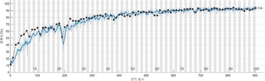
In the equation, V defines the new sequence, and S defines the existing sequence. β is a hyperparameter with a value between 0 and 1. Figures 8 and 9 show the training accuracy and loss graphs, respectively. As a result of the training, accuracy was achieved at epoch 2, and the training was terminated.

Figure 8:

Accuracy graph

Figure 9:

Loss graph

The training results are shown in Table 5 below.

Table 5:

Training results

The training of this model was conducted for a total of 100 epochs. With 9 iterations per epoch, a total of 900 iterations were performed throughout the entire training process.

5. Simulation Results

To verify the final performance of the trained model, an evaluation was conducted using the 255 test data images partitioned in Chapter 4 as inputs for the classification algorithm. As a result, 244 out of 255 images were correctly classified, achieving an accuracy of 95.69%.

In addition to simple accuracy, Precision, Recall, and F1-score were calculated based on a confusion matrix for a more multifaceted evaluation of the algorithm's performance. Among these, Precision refers to the ratio of actual positive samples among those predicted as positive by the model. It is a key metric for evaluating the accuracy of model predictions and is calculated as shown in Equation (4).

Here, True Positive (TP) represents the number of cases where actual positive data was correctly predicted as positive, and False Positive (FP) denotes the number of cases where actual negative data was incorrectly predicted as positive. High precision indicates a high ratio of actual positive data among the results identified as positive by the model, making it a critical metric in environments where the occurrence of FPs must be minimized.

Next, Recall represents the proportion of actual positive samples that the model correctly detected as positive. This serves as a measure to evaluate the model's practical target detection capability and is calculated as shown in Equation (5).

Here, FN refers to False Negative, which indicates the misclassification of actual positive data as negative. Recall signifies the ability to correctly detect actual positive samples and is an important criterion in models where minimizing false negatives is required.

Finally, the F1-score represents the harmonic mean of precision and recall. This metric yields a high value when both precision and recall are balanced and excellent, and it is used to assess the overall performance of the model. Its calculation formula is shown in Equation (6)[9].

The F1-score is calculated by dividing the product of precision and recall by their sum and then multiplying by 2. This prevents the metric from being biased toward either precision or recall and is useful for comprehensively judging balanced performance between the two evaluation criteria. The F1-score ranges from 0 to 1, with a value closer to 1 indicating superior predictive performance of the model.

Figure 10 shows the confusion matrix derived from this study. Based on this matrix, precision is calculated as the ratio in the column direction (predicted values), and recall is calculated as the ratio in the row direction (actual values).

Figure 10:

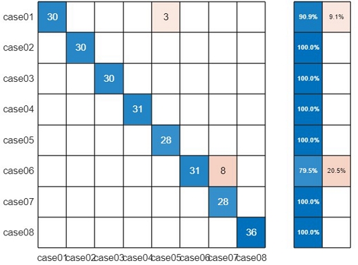
Confusion matrix

The precision, recall, and F1-score for each case calculated based on the confusion matrix are shown in Table 6 below.

Table 6:

Calculation of precision, recall, and F1-score

As a result of the calculations, the model's average precision was 0.960, the average recall was 0.963, and the average F1-score was 0.958, confirming that the classification algorithm proposed in this study possesses excellent performance. While some misclassifications occurred in Case 1 and Case 6, most other cases exhibited high classification accuracy approaching 100%. The combined fault scenario (Case 6) exhibited a relatively low recall of 79.5%, often being misclassified into Case 7. Qualitatively, this is attributed to the overlapping damping effects of both internal leakage and friction on the transient pressure signals. However, a rigorous quantitative segregation of these coupled physical mechanisms remains a limitation of the current simulation setup. Further data-driven analysis through isolated parameter variations and experimental validation will be systematically conducted in our follow-up research to clarify this misclassification phenomenon.

6. Conclusion

In this study, a hybrid-based fault diagnosis methodology was proposed and its effectiveness was verified for the Rotor Sail system, an eco-friendly auxiliary ship propulsion device gaining attention following the strengthening of environmental regulations by the International Maritime Organization (IMO). The methodology aims to overcome the problem of insufficient failure data encountered during the initial introduction stage of such equipment. To this end, an FMEA analysis based on the international standard (IEC 60812) was first performed, identifying the hydraulic cylinder of the tilting structure—which can lead to catastrophic accidents such as overturning in the event of failure—as the core diagnostic target with the highest failure risk.

To overcome the fundamental limitation of lacking failure data in actual industrial sites, this study constructed a physical model using MATLAB Simulink to simulate the dynamic behavior of the target hydraulic cylinder. Through this, a total of eight state classes were defined, including normal states as well as possible leakage and friction defects, and 1,710 virtual time-series failure datasets were generated through repeated simulations. The acquired 1D time-series signals were pre-processed into 2D Scalogram images using the Continuous Wavelet Transform (CWT) technique, which effectively captures the transitional characteristics of abnormal signals, and were converted into a dataset for deep learning training.

The constructed image dataset was applied to GoogLeNet, a pre-trained convolutional neural network (CNN) model, through transfer learning to complete the final fault diagnosis classification algorithm. Evaluating the final performance of the trained model using independent test data—which was strictly excluded from the training and validation processes—resulted in an excellent classification accuracy of 95.69%. Furthermore, evaluation metrics based on the confusion matrix, calculated to verify the multifaceted performance of the model, recorded an average precision of 0.960, an average recall of 0.963, and an average F1-score of 0.958, proving that defects can be diagnosed with high reliability even for complex failure modes.

In conclusion, the fault diagnosis methodology proposed in this study, which integrates physical simulation modeling and deep learning algorithms, can serve as a promising baseline for preemptively establishing Condition-Based Maintenance (CBM) systems for new marine equipment where actual failure data is difficult to obtain due to short operational histories. Nevertheless, this study possesses a technical limitation in that dynamic environmental variables—such as ship-motion effects, operational wind loads, and hydraulic-oil temperature fluctuations—were excluded from the simulation, as the tilting mechanism primarily operates under berthed conditions. Therefore, to expand the practical applicability of the proposed framework to real-world continuous monitoring, incorporating these multi-physics environmental variables and conducting onboard experimental validations remain essential. Future research plans include applying the diagnostic model developed through this study to scale-model experimental devices or Rotor Sail systems on ships currently operating at sea, thereby further enhancing the field applicability and robustness of the algorithm through cross-validation with measured data.

Acknowledgments

This work was supported by the Technology Innovation Program (20024863, Development of demonstration technology for wind power propulsion system for ship operation energy saving) funded By the Ministry of Trade Industry & Energy(MOTIE, Korea)

References

• International Maritime Organization, Draft Report of the Marine Environment Protection Committee on its Eightieth Session, MEPC 80/WP.1, Marine Environment Protection Committee, UK, 2023.
• UMAS, An Overview of the Discussions from IMO MEPC 80 and Frequently Asked Questions, https://www.u-mas.co.uk, , Accessed April 17, 2026.
• International Maritime Organization, International Maritime Organization (IMO) adopts revised strategy to reduce greenhouse gas emissions from international shipping, https://www.imo.org, , Accessed April 17, 2026.
• K. Jenab, J. Ortega-Moody, and S. Staub, “A comprehensive review of machine learning techniques for condition-based maintenance,” International Journal of Prognostics and Health Management, vol. 15, no. 2, 2024. [https://doi.org/10.36001/ijphm.2024.v15i2.3850]
• L. Das, B. Gjorgiev, and G. Sansavini, “Uncertainty-aware deep learning for monitoring and fault diagnosis from synthetic data,” Reliability Engineering & System Safety, vol. 251, p. 110386, 2024. [https://doi.org/10.1016/j.ress.2024.110386]
• H. F. Losada, S. V. Machin, and F. M. Montero, “Bearing fault diagnosis: An efficient architecture based on CNN and transfer learning,” Proceedings of IEEE URUCON, pp. 392-396, 2024. [https://doi.org/10.1109/URUCON63440.2024.10850037]
• International Electrotechnical Commission, "Failure modes and effects analysis (FMEA) and failure modes, effects and criticality analysis (FMECA)," Switzerland, IEC Standard 60812, 2018.
• C. Szegedy, W. Liu, Y. Jia, P. Sermanet, S. Reed, D. Anguelov, D. Erhan, V. Vanhoucke, and A. Rabinovich, “Going deeper with convolutions,” Proceedings of the IEEE Conference on Computer Vision and Pattern Recognition, pp. 1-9, 2015. [https://doi.org/10.1109/CVPR.2015.7298594]
• B. S. Kang and C. H. Jung, “A study on the development of YOLO-based maritime object detection system through geometric interpretation of camera images,” Journal of the Korean Society of Marine Environment & Safety, vol. 28, no. 4, pp. 499-506, 2022. [https://doi.org/10.7837/kosomes.2022.28.4.499]