The Korean Society of Marine Engineering

[ Original Paper ]

Journal of Advanced Marine Engineering and Technology - Vol. 48, No. 1, pp.24-31

ISSN: 2234-7925 (Print) 2765-4796 (Online)

Print publication date 29 Feb 2024

Received 10 Jan 2024 Revised 26 Jan 2024 Accepted 15 Feb 2024

DOI: https://doi.org/10.5916/jamet.2024.48.1.24

Discrete stochastic EOQ model for deteriorating inventory in supply chain using Hamilton–Jacobi–Bellman equation

Long Le Ngoc Bao¹ ; Sam-Sang You² ; Hwan-Seong Kim^†

1Ph. D. Candidate, Department of Logistics, Korea Maritime & Ocean University baolong@g.kmou.ac.kr
2Professor, Division of Mechanical Engineering, Korea Maritime & Ocean University ssyou@kmou.ac.kr

Correspondence to: ^†Professor, Department of Logistics, Korea Maritime & Ocean University, 727, Taejong-ro, Yeongdo-gu, Busan 49112, Korea, E-mail: kimhs@kmou.ac.kr, Tel: +82-51-410-4334

Copyright © The Korean Society of Marine Engineering
This is an Open Access article distributed under the terms of the Creative Commons Attribution Non-Commercial License (http://creativecommons.org/licenses/by-nc/3.0), which permits unrestricted non-commercial use, distribution, and reproduction in any medium, provided the original work is properly cited.

Abstract

In an ideal environment, an optimal replenishment point is required for the best output performance with maximized profit for a classical economic order quantity (EOQ) model. However, in practice, most supply chains experience variations that affect the theoretical results. Most products are perishable, which implies that their quality deteriorates over time. This issue must be resolved promptly before the cycle ends because unsold items result in revenue loss. This study presents an EOQ model in a discrete domain with uncertainties in the systematic parameters. The demand for products depends linearly on the pricing scheme of the enterprise, which must be analyzed optimally to achieve the maximum profit in the replenishment cycle. To solve this optimization problem, an optimal control technique named the Hamilton–Jacobi–Bellman (HJB) equation is introduced, which has been proven successful in solving similar issues. The convergence constraints of the HJB equation and the optimal reordering quantity are analyzed. The performance of the proposed approach is revealed via simulations, in which the behavior of the inventory system in perfect and imperfect scenes is demonstrated. The final result indicates that the optimal solution is admissible and robust as it remains valid in varying environments, with a difference of less than 5% in the ideal case.

Keywords:

Inventory management, EOQ model, Deteriorating products, Parametric variations, HJB equation

1. Introduction

Inventory management is crucial in commerce. The primary aim of inventory management is to minimize the overall system cost via informed decision-making based on various mathemati-cal methodologies such as optimal control analysis, dynamic programming, and network optimization. Inventory decisions determine the optimal timing for replenishment and the quantity to be added. The core objective of inventory theory is to identify managerial guidelines for reducing inventory expenses while fulfilling market demands. To achieve the optimal total cost using an inventory model, most industrial entities emphasize inventory control and strive to navigate challenges such as managing and sustaining stocks of perishable items. The concept of deteriora-tion, which encompasses various forms of damage, spoilage, dryness, and vaporization [1], is crucial in the management of inventory models. Deterioration is important in inventory analy-sis, as it affects cost reduction and profit maximization. Failure to remove degraded items from a system can significantly affect inventory operations. Without relevant monitoring, deterioration will cause excessive waste and losses, which may reach up to 30% in some countries [2]-[3]. In recent decades, researchers have focused primarily on controlling and sustaining inventories. In practical scenarios, item decay or deterioration is natural and evident in various products such as vegetables, fruits, foods, perfumes, chemicals, pharmaceuticals, radioactive substances, and electronic equipment.

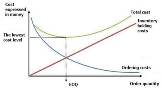
Many businesses prioritize inventory management and trou-bleshooting inventory issues to achieve the economic order quan-tity (EOQ), which minimizes the overall average inventory costs. Generally, for deteriorating products, the inventory decays over time, thus causing profit losses because the degraded items can-not be sold and must be removed from the stock. Unsold items in the inventory increase the holding costs over time until all items are depleted, whereas the ordering cost decreases over time. The aggregated cost features an optimum point at which replenish-ment minimizes the overall cost, as illustrated in Figure 1.

Figure 1:

General concept of EOQ in supply chain

The foundational inventory model for deteriorating items as-serts that inventory depletion primarily stems from a consistent demand rate. Whitin [4] examined the effect of deterioration on fashion items once they surpassed the recommended date. Wag-ner and Whitin [5] introduced a dynamic version of the classical EOQ model developed for deteriorating items. Ghare and Schrader [6] investigated an inventory model for deteriorating items, which was characterized by constant deterioration and demand rates. Shah and Jaiswal [7] investigated an order-level inventory model developed for deteriorating items at a constant deterioration rate. Aggarwal [8] expanded Shah and Jaiswal’s work by calculating the average holding cost. Dave and Patel [9] developed an inventory model for deteriorating items character-ized by linearly increasing demand and deterioration rates, which remained a constant fraction of the on-hand inventory. All the aforementioned models were developed based on constant deteri-oration rates, constant demand rates, infinite replenishment, and no shortages. Heng et al. [10] introduced an exponentially decay-ing inventory model for deteriorating items by assuming a finite replenishment rate and constant demand rate. Reviews summariz-ing advancements in deteriorating inventory are available in the literature [11]-[15].

Pricing policy is widely recognized as one of the most preva-lent and effective methods in businesses for influencing customer demand. As mentioned in [16], realizing optimal pricing policies can offer competitive advantages to firms. Many studies have approached pricing policies as an optimization problem to max-imize the expected cumulative profit, where the pricing strategy was prioritized in the objective function. The Hamilton–Jacobi–Bellman (HJB) equation has been proposed in numerous studies, either in a continuous or discrete domain, as a robust optimization tool to yield an analytical solution [17]-[20].

The HJB equation has been widely applied in many previous studies, particularly in continuous models using the analytical approach. In the case of deterministic problems, for instance, Dye’s model [21] formulates customer demand as a multiplicative function comprising price, the advertising goodwill, and a fresh-ness index. Yang and Zhang [22] used the HJB equation for the EOQ model, where stationary demand was expressed in a mul-tinominal logit (MNL) model, along with inventory-cost and inventory penalty functions. Furthermore, the MNL model was used to derive a deterministic relaxation formulation for station-ary demand [23]. Recently, stochastic problems have been inves-tigated extensively as they can describe issues more realistically. In such problems, customer demand is typically expressed as a stochastic process, such as the Poisson process [24], Brownian motion [25], or Bernoulli random variable [23]. However, most studies focused on stochastic events instead of variations in sys-tematic parameters as a source of uncertainty. Most real-world systems are difficult to model owing to the change in parameters over time. To describe the behavior of these systems precisely, one should consider the effect of parametric variation.

Hence, this study is performed to address the research gap mentioned above by introducing a discrete stochastic deteriorat-ing inventory model based on the EOQ concept, whose deteriora-tion rate is uniformly distributed in a specified range. Customer demand is assumed to depend on a product’s price as a linear function with varying coefficients over time. Within this uncer-tain environment, the final objective is to craft an optimal policy that maximizes the total cumulative profit, as well as to realize the replenishment quantity for every cycle. The main contributions of this study are as follows:

① A stochastic model for an inventory system is constructed, which includes uncertainties in the deterioration rate and the coefficients of the demand function.
② An analytical solution for achieving the optimal pricing using the HJB equation is derived comprehensively.
③ The solution convergence and the optimal replenishment quantity are analyzed.
④ Numerical simulations are conducted to reveal the perfor-mance of the proposed policy and compare the outputs in ideal and uncertain scenarios.

The remainder of this paper is organized as follows: Section 2 describes the proposed inventory system using a mathematical model. Section 3 provides a detailed analysis of the convergence condition of the solution, including the closed forms of the coef-ficients and the compact form of the optimal pricing policy, as well as the best quantity to be replenished per cycle. Simulations performed to validate the analytical results are presented in Section 4, and Section 5 concludes the paper.

2. Problem Description & Modeling

2.1 Problem Description

In the EOQ model, quantity total of Q0 units are replenished at the beginning of the replenishment cycle. The stock decays over time until no items remain in the inventory, which implies that all the items must be sold promptly for the maximum profit; this is because deteriorated items are not sold and thus do not profit the supply chain. Customer demand is governed by the product price; therefore, a good pricing scheme is required to manipulate product flow. As replenishment occurs only once per cycle, the pricing of products should account for the cycle length, as a stockout negates the demand and does not provide any income. The inventory level must be controlled such that it ends at the end of the cycle to maximize the total profit. In practice, owing to the numerous sources of uncertainty in the system, managing cus-tomer demand is difficult and the stock is typically depleted be-fore a new cycle begins, thus reducing the profit compared with the ideal case. The key annotations used herein are listed in Table 1.

Table 1:

Annotation of key variables used herein

2.2 Problem Modeling

Consider a single replenishment cycle of inventory control with length T. The model is developed in a discrete domain as follows: The inventory level (n+1) of a product depends on the deterioration rate θ(n) and demand d(n), as expressed in the fol-lowing equation:

I n + 1 = 1 - θ n I n - d n

(1)

where θ(n) is an unknown term and bounded in [0,θ₀] with θ₀<1.. In addition, demand is a stochastic term resulting from the product’s pricing policy, which is assumed to have the following linear relationship:

n = a^n - b^n p n

(2)

where $a^n$ and $b^n$ are positive coefficients distributed around the nominal values a and b respectively; that is, $E a^n = a$ and $E b^n = b$ . The cycle length is determined by the moment the inventory level reaches zero.

T = sup ⁡ n ∈ N + | I n ≥ 0

(3)

Because θ(n) is unknown, one can assume that θ(n) is uniformly distributed in the range [0,θ₀] and features an expectation of $E θ n = θ 0 2$ . Moreover, the expected demand at every time instance n is only determined by the pricing policy p(n), i.e., $E d n ≜ a - b p (n)$ . Hence, by considering $x n ≜ E I n$ and $θ 1 ≜ 1 - θ 0 2$ , Equation (1) can be rewritten as

n + 1 = θ 1 x n - a + b p n

(4)

Consequently, the following analytical solution is obtained:

x n = θ 1 n Q 0 - a 2 1 - θ 1 n Q 0 + b ∑ i = 0 n - 1 θ 1 n - 1 - i p i

(5)

In the next section, we determine the expectation of the optimal pricing policy using the HJB equation.

2.3 HJB equation

Hereinafter, simplified notations $x n ≡ x (n)$ , $p n ≡ p (n)$ , and $d n ≡ d (n)$ will be used for ease of description. The expected profit rate function L(_xn) resulting from the sales revenue is expressed as follows:

L x n ≜ p n d n = p n a - b p n

(6)

Subsequently, the expected optimal profit obtained from the time instance n < T until T is expressed as

V x n ≜ s u p ⁡ ∑ i = n T - 1 L x i

(7)

Using the Bellman’s principle of optimality, the HJB equation is obtained directly from Equation (7) as

V x n = sup ⁡ L x n + V x n + 1 = sup p . ⁡ p n a - b p n + V x n + 1

(8)

Apply partial derivative and chain rule for both side of Equation (8) with $v x n ≜ ∂ V (x n) ∂ x n$ , the optimal price function $p n *$ is the solution of the following equation:

∂ ∂ p n V x n = a - 2 b p n + b v x n + 1 = 0

(9)

which finally obtains

p n * = a 2 b + 12 v x n + 1

(10)

Most previous studies used the quadratic form of V(x_n), i.e., $V x n = γ n + α n x n + β x n 2$ , where $(γ n, α n, β n) ∈ R$ are coefficients that may vary over time. Substituting the coefficients into Equation (10) yields the following equations:

x n + 1 = θ 1 x n - a + b p n * = θ 1 1 - b β n + 1 x n + - a + b α n + 1 2 1 - b β n + 1 .

(11)

v x n + 1 = α n + 1 + 2 β n + 1 x n + 1 = 2 θ 1 β n + 1 1 - b β n + 1 x n + α n + 1 - a β n + 1 1 - b β n + 1 .

(12)

p n * = a 2 b + 12 v x n + 1 = a 2 b + α n + 1 - a β n + 1 2 1 - b β n + 1 + θ 1 β n + 1 1 - b β n + 1 x n

(13)

V x n + 1 = γ n + 1 + α n + 1 x n + 1 + β n + 1 x n + 1 2 = β n + 1 θ 12 1 - b β n + 1 2 x n 2 + α n + 1 θ 1 1 - b β n + 1 + - a + b α n + 1 β n + 1 θ 1 1 - b β n + 1 2 x n + γ n + 1 + α n + 1 - a + b α n + 1 2 1 - b β n + 1 + β n + 1 - a + b α n + 1 2 4 1 - b β n + 1 2 .

(14)

Also, expanding V(x_n) and then simplifying would yield

V x n = β n + 1 θ 12 1 - b β n + 1 x n 2 + - H + θ 1 α n + 1 - a θ 1 β n + 1 1 - b β n + 1 x n + + γ n + 1 + a 2 - 2 a b α n + 1 + b 2 α n + 1 2 4 b 1 - b β n + 1

(15)

After some computation steps, the series {γ_n}, {α_n}, and {β_n} can be determined via the following recursive relationships:

γ n + 1 = γ n - a θ 1 - b α n 2 4 b θ 12 + b β n

(16)

α n + 1 = θ 1 α n + a β n θ 12 + b β n

(17)

β n + 1 = β n θ 12 + b β n

(18)

The closed-form expressions for the series in Equations (16), (17), and (18), as well as the estimate for the replenishment cycle T are derived in detail in the following section.

3. Convergence Condition & Optimal Replenishment Quantity

3.1 Convergence Condition for Optimal Solution

The finite series {γ_n}, {α_n}, and {β_n} should be determined such that the state x_n will finally converge. In addition, the quadratic form of V(x_n) should be concave, i.e., β_n is negative for all n∈[0,T]. Based on Equations (16), (17), and (18), the following conditions must hold:

β n < 0 1 - β n > θ 1 θ 12 + b β n > 0 ∀ n ∈ 0, T

(19)

Solving Equation (19) leads to

- θ 12 b < β n < 0 ∀ n ∈ 0, T

(20)

Furthermore, we obtain

β n + 1 - β n = β n 1 - θ 12 - b β n θ 12 + b β n < 0 ∀ β n ∈ - θ 12 b, 0

(21)

Hence, $β n + 1 - β n < 0 ∀ n ∈ [0, T]$ , which implies that {β_n} is a monotonically decreasing sequence and $β n → - θ 12 b$ as n→∞. The closed-forms of {α_n} and {β_n} are presented in Proposition 1 below.

Proposition 1: The closed-forms of {α_n} and {β_n} are as follows:

β n = β 0 θ 1 2 n + b β 0 ∑ i = 0 n - 1 θ 1 2 i α n = θ 1 n α 0 + a β 0 ∑ i = 0 n - 1 θ 1 i θ 1 2 n + b β 0 ∑ i = 0 n - 1 θ 1 2 i .

(22)

Proof: This proof is obtained through induction. It is clear that

β 1 = β 0 θ 12 + b β 0 α 1 = θ 1 α 0 + a β 0 θ 12 + b β 0 .

(23)

Next, assume that Equation (23) holds for $n = m ∈ [0, T - 1]$ . As such,

β m + 1 = β m θ 12 + b β m = β 0 θ 1 2 m + b β 0 ∑ i = 0 m - 1 θ 1 2 i θ 12 + b β 0 θ 1 2 m + b β 0 ∑ i = 0 m - 1 θ 1 2 i = β 0 θ 12 (θ 1 2 m + b β 0 ∑ i = 0 m - 1 θ 1 2 i) + b β 0 = β 0 θ 1 2 (m + 1) + b β 0 ∑ i = 0 m θ 1 2 i .

(24)

Therefore, the closed-form of {β_n} is proved. Using this result yields

α m + 1 = θ 1 α m + a β m θ 12 + b β m = θ 1 θ 1 m α 0 + a β 0 ∑ i = 0 m - 1 θ 1 i θ 1 2 m + b β 0 ∑ i = 0 m - 1 θ 1 2 i + a β 0 θ 1 2 m + b β 0 ∑ i = 0 m - 1 θ 1 2 i θ 12 + b β 0 θ 1 2 m + b β 0 ∑ i = 0 m - 1 θ 1 2 i = θ 1 m + 1 α 0 + a β 0 ∑ i = 1 m θ 1 i + a β 0 θ 12 (θ 1 2 m + b β 0 ∑ i = 0 m - 1 θ 1 2 i) + b β 0 = θ 1 m + 1 α 0 + a β 0 ∑ i = 0 m θ 1 i θ 1 2 (m + 1) + b β 0 ∑ i = 0 m θ 1 2 i .

(25)

Based on induction, the closed-form of {α_n} is proved as well. Because $0 ≤ θ 1 < 1, θ 1 n → 0 a n d θ 1 2 n → 0 a s n → T$ . Therefore, the closed-form of {γ_n} is approximated by excluding the high-order exponent terms of θ₁. Hence,

θ 12 + b β n = θ 12 + b β 0 θ 1 2 n + b β 0 ∑ i = 0 n - 1 θ 1 2 i ≈ θ 12 + b β 0 b β 0 1 1 - θ 12 = 1 .

(26)

a θ 1 - b α n = a θ 1 - b θ 1 n α 0 + a β 0 ∑ i = 0 n - 1 θ 1 i θ 1 2 n + b β 0 ∑ i = 0 n - 1 θ 1 2 i ≈ a θ 1 - b a β 0 1 1 - θ 1 b β 0 1 1 - θ 12 = a θ 1 - a 1 - θ 12 1 - θ 1 = - a .

(27)

Thus:

γ n + 1 = γ n - a θ 1 - b α n 2 4 b (θ 12 + b β n) ≈ γ n - a 2 4 b

(28)

Finally, the closed-form of {γ_n} is

γ n = γ 0 - n a 2 4 b

(29)

Replacing the achieved results into Equation (13) leads to the compact form of optimal pricing $p n *$ as

p n * = a 2 b + α n 2 θ 1 + β n θ 1 x n

(30)

3.2 Optimal Replenishment Quantity

Based on the optimal pricing policy obtained and the replenishment quantity Q0, the maximum expected profit in a replenishment cycle can be calculated as $V Q 0 = γ 0 + α 0 Q 0 + β 0 Q 02$ . Because β₀ < 0, we have $max ⁡ V Q 0 = γ 0 - α 02 4 β 0$ when $Q 0 = - α 0 2 β 0$ . Owing to the definition of the replenishment cycle, V(x_T)=0 as x_T→0, which indicates that γ_T→0. Applying this to Equation (29) yields the following expression for the replenishment cycle:

T = 4 b γ 0 a 2 .

(31)

Thus, the optimal replenishment quantity and cycle can be computed based on pricing policy coefficients. Simulation results are presented in the next section to verify the performance of the proposed approach.

4. Simulation Results

4.1 Context, Assumptions, and Parameters used

Numerical simulations were conducted to verify the perfor-mance of the proposed optimal pricing policy. Based on a prede-fined replenishment cycle, the pricing policy should be able to maximize the total expected profit and control the inventory level to ensure no stockout until the end of the cycle. The simulation parameters are listed in Table 2.

Table 2:

Parameters used in current simulation

In addition, the following assumptions were introduced in the simulation:

① Replenishment is performed only once at the beginning of the cycle. For the remainder of the cycle, the inventory lev-el is only affected by the customer demand and deterioration.
② If stockouts occurs, then no further demand exists until the end of the cycle.
③ The expected values are computed using nominal values (deterministic values), whereas the varying values are av-eraged from 10 trials using random values obtained from the distribution (stochastic values).

4.2 Optimal Pricing for Predefined Replenishment Cycle

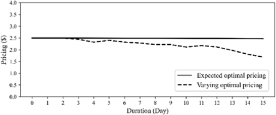
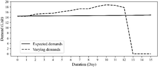
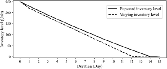
For a cycle length T=15 and an initial quantity estimated as $Q 0 = - α 0 2 β 0 = 250$ , as shown in Table 2, the optimal pricing is realized in the compact form shown in Equation (30). The sequences {α_n,β_n,γ_n} are computed in the closed forms shown in Equations (22) and (29), where $γ 0 = a T 2 4 b$ , as obtained using Equation (31). The expected inventory level is calculated recursively using Equation (11). Figures 2, 3, and 4 show the optimal pricing policy, expected demand, and inventory level, respectively, where one can compare the values in a stochastic environment with varying values of $a^, b^, θ$ .

Figure 2:

Optimal pricing policy in ideal and varying cases

Figure 3:

Customer demand in ideal and varying cases

Figure 4:

Inventory level in ideal and varying cases

As shown, in the ideal case, the optimal pricing manages to manipulate the inventory level such that the stock will be sold out at the end of the cycle, whereas in the realistic case, the inventory is depleted sooner owing to the variations of several parameters $a^, b^, θ$ . The optimal pricing was preserved during the cycle; however, in the stochastic environment, it decreased by day. The demand increases accordingly, making the inventory finished earlier. This is as expected because, in practice, many unexpected events and changes occur during the sale and the inventory will be depleted earlier than expected.

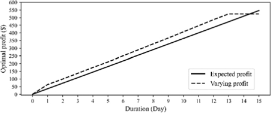
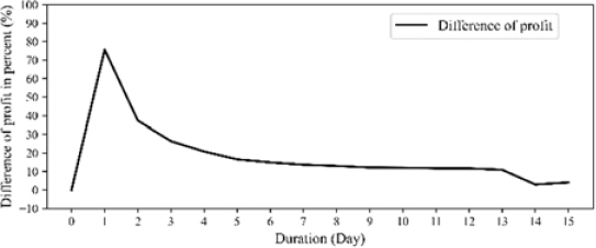
To obtain deeper insights, the total profits obtained in the ideal and stochastic cases were compared, as shown in Figure 5. As the demand in a stochastic environment is typically greater than that in an ideal environment, the profit at the beginning of the former environment is slightly higher. However, the inventory is depleted sooner, thus rendering the total cumulative profit less than that in the perfect scenario. Figure 6 shows the difference in profit for the two cases in terms of percentage. The difference peaked at approximately 80% at the beginning but reduced grad-ually until the end of the cycle, where the final error was meas-ured at 4.493%, which was admissible in a complex environment with various changes during operation. Ultimately, the robustness of the proposed pricing policy was reflected as the total cumula-tive profit in a complicated scenario does not differ significantly from that in a perfect scenario. Therefore, based on this finding, managers can devise an optimal solution for a volatile supply chain and adjust the pricing policy to maximize the profit in a predefined replenishment cycle.

Figure 5:

Comparison of cumulative profit between two environments

Figure 6:

Difference in profit (in percentage) between two environments

5. Conclusion

In this study, an optimal control technique for a discrete EOQ-decaying inventory system was applied using the HJB equation to maximize the cumulative profit. The proposed pricing policy is robust for cases involving oscillating parameters and complex environments, as the difference in profit between the output in ideal and realistic scenarios remains under 5%. For a specified replenishment cycle length, the proposed method provided an optimal pricing that maximized the profit, even under imperfect conditions. The pricing policy significantly affects an enterprise’s profit. Therefore, the proposed technique is promising for deci-sion makers as it can yield the best policy under predefined oper-ating conditions and markets, even for volatile ones.

In this study, all unknown and variation sources of the supply chain were reflected in the model as oscillations of systematic parameters. In addition, customer demand was modeled as a linear function of pricing, which may not be suitable for practical cases as more factors affect customer behavior in reality. In the future, this study can be expanded by adding realistic constraints. For instance, the selection of customers, which is typically un-predictable and randomized, can be modeled stochastically. This renders the study more practical and highlights the robustness of optimal control methods.

Acknowledgments

This research was supported by “Regional Innovation Strategy (RIS)” through the National Research Foundation of Korea (NRF) funded by the Ministry of Education (MOE)(2023RIS007).

Author Contributions

Conceptualization, L. N. B. Long and S. S. You; Methodology, L. N. B. Long; Software, L. N. B. Long; Validation, S. S. You and H. S. Kim; Formal Analysis, L. N. B. Long; Investigation, L. N. B. Long; Resources, L. N. B. Long; Data Curation, L. N. B. Long; Writing—Original Draft Preparation, L. N. B. Long; Writing—Review & Editing, S. S. You and H. S. Kim; Visualization, L. N. B. Long; Supervision, H. S. Kim; Project Administration, H. S. Kim; Funding Acquisition, H. S. Kim.

References

X. Pan and S. Li, “Optimal control of a stochastic production-inventory system under deteriorating items and environmental constraints,” International Journal of Production Research, vol. 53, no. 2, pp. 607-628, 2015. [https://doi.org/10.1080/00207543.2014.961201]
X. Cai, J. Chen, Y. Xiao, and X. Xu, “Optimization and coordination of fresh product supply chains with freshness-keeping effort,” Production and Operations Management, vol. 19, no. 3, pp. 261-278, 2010. [https://doi.org/10.1111/j.1937-5956.2009.01096.x]
Y. Yang, H. Chi, W. Zhou, T. Fan, and S. Piramuthu, “Deterioration control decision support for perishable inventory management,” Decision Support Systems, vol. 134, 2020. [https://doi.org/10.1016/j.dss.2020.113308]
T. M. Whitin, The Theory of Inventory Management, 2nd edition: Princeton University Press, 1957.
H. M. Wagner and T. M. Whitin, “Dynamic version of the economic lot size model,” Management Science, vol. 5, no. 1, pp. 89-96, 1958. [https://doi.org/10.1287/mnsc.5.1.89]
P. M. Ghare and G. F. Schrader, “A model for an exponentially decaying inventory,” Journal of Industrial Engineering, vol. 14, pp. 238-243, 1963.
Y. K. Shah, and M. C. Jaiswal, “An order-level inventory model for a system with constant rate of deterioration,” Opsearch, vol. 14, no. 3, pp. 174-184, 1977.
S. P. Aggarwal, “A note on an order-level inventory model for a system with constant rate of deterioration,” Opsearch, vol. 15, no. 4, pp. 184-187, 1978.
U. Dave and L. K. Patel, “(T, Si) policy inventory model for deteriorating items with time proportional demand,” Journal of the Operational Research Society, vol. 32, no. 2, pp. 137-142, 1981. [https://doi.org/10.1057/jors.1981.27]
K. J. Heng, J. Labban, and R. J. Linn, “An order-level lot-size inventory model for deteriorating items with finite replenishment rate,” Computers & Industrial Engineering, vol. 20, no. 2, pp. 187-197, 1991. [https://doi.org/10.1016/0360-8352(91)90024-Z]
F. Raafat, “Survey of literature on continuously deteriorating inventory models,” Journal of the Operational Research Society, vol. 42, no. 1, pp. 27-37, 1991. [https://doi.org/10.1057/jors.1991.4]
S. K. Goyal and B. C. Giri, “Recent trends in modeling of deteriorating inventory,” European Journal of Operational Research, vol. 134, no. 1, pp. 1-16, 2001. [https://doi.org/10.1016/S0377-2217(00)00248-4]
R. Li, H. Lan, and J. R. Mawhinney, “A review on deteriorating inventory study,” Journal of Service Science and Management, vol. 3, no, 1, pp. 117-129, 2010. [https://doi.org/10.4236/jssm.2010.31015]
M. Bakker, J. Riezebos, and R. H. Teunter, “Review of inventory systems with deterioration since 2001,” European Journal of Operational Research, vol. 221, no. 2, pp. 275-284, 2012. [https://doi.org/10.1016/j.ejor.2012.03.004]
L. Janssen, T. Claus, and J. Sauer, “Literature review of deteriorating inventory models by key topics from 2012 to 2015,” International Journal of Production Economics, vol. 182, pp. 86-112, 2016. [https://doi.org/10.1016/j.ijpe.2016.08.019]
A. V. den Boer, “Dynamic pricing and learning: Historical origins, current research, and new directions,” Surveys in Operations Research and Management Science, vol. 20, no. 1, pp. 1-18, 2015. [https://doi.org/10.1016/j.sorms.2015.03.001]
C. Y. Dye, “Optimal joint dynamic pricing, advertising and inventory control model for perishable items with psychic stock effect,” European Journal of Operational Research, vol. 283, no. 2, pp. 576-587, 2020. [https://doi.org/10.1016/j.ejor.2019.11.008]
T. Fan, C. Xu, and F. Tao, “Dynamic pricing and replenishment policy for fresh produce,” Computers & Industrial Engineering, vol. 139, 2020. [https://doi.org/10.1016/j.cie.2019.106127]
J. Chen, M. Dong, Y. Rong, and L. Yang, “Dynamic pricing for deteriorating products with menu cost,” Omega, vol. 75, pp. 13-26, 2018. [https://doi.org/10.1016/j.omega.2017.02.001]
Y. Duan, Y. Cao, and J. Huo, “Optimal pricing, production, and inventory for deteriorating item under demand uncertainty: The finite horizon case,” Applied Mathematical Modelling, vol. 58, pp. 331-348, 2018. [https://doi.org/10.1016/j.apm.2018.02.004]
C.Y. Dye, “Optimal joint dynamic pricing, advertising and inventory control model for perishable items with psychic stock effect,” European Journal of Operational Research, vol. 283, no. 2, pp. 576-587, 2020. [https://doi.org/10.1016/j.ejor.2019.11.008]
N. Yang and R. Zhang, “Comparative statics analysis of an inventory management model with dynamic pricing, market environment fluctuation, and delayed differentiation,” Production and Operations Management, vol. 31, no. 1, pp. 341-357, 2022. [https://doi.org/10.1111/poms.13538]
Y. -W. Zhou, X. Zhang, Y. Zhong, B. Cao, and T. C. Edwin Cheng, “Dynamic pricing and cross-channel fulfillment for omnichannel retailing industry: An approximation policy and implications,” Transportation Research Part E: Logistics and Transportation Review, vol. 156, 2021. [https://doi.org/10.1016/j.tre.2021.102524]
Y. Chen and V. F. Farias, “Robust dynamic pricing with strategic customers,” Mathematics of Operations Research, vol. 43, no. 4, pp. 1119-1142, 2018. [https://doi.org/10.1287/moor.2017.0897]
Y. Duan, Y. Cao, and J. Huo, “Optimal pricing, production, and inventory for deteriorating items under demand uncertainty: The finite horizon case,” Applied Mathematical Modelling, vol. 58, pp. 331-348, 2018. [https://doi.org/10.1016/j.apm.2018.02.004]

Annotation	Definition
n	Time instances in the discrete domain
I(n)	Inventory level at time n
x(n)	Expected inventory level at time n
d(n)	Demand quantity at time n
p(n)	Product’s price at time n
Q₀	Replenishment quantity per cycle
a, b	Coefficients of demand function
α_n, β_n, γ_n	Coefficients of the accumulative profit function

Parameter	Value	Unit
T	15	Days
θ₀	0.05	-
a	50	-
b	10	-
α₀	0.05	-
β₀	-0.0001	-