Experimental study on predicting the corrosion behavior of carbon steel in various corrosive environments using artificial neural networks
Copyright © The Korean Society of Marine Engineering
This is an Open Access article distributed under the terms of the Creative Commons Attribution Non-Commercial License (http://creativecommons.org/licenses/by-nc/3.0), which permits unrestricted non-commercial use, distribution, and reproduction in any medium, provided the original work is properly cited.
Abstract
In this study, potentiodynamic polarization curves of carbon steel were employed to systematically characterize and predict its electrochemical corrosion behavior under varying environmental conditions. A three-factor full factorial design was utilized to vary critical parameters such as temperature, pH, and salinity, simulating diverse marine conditions. Using the TensorFlow 2.0 framework, a model based on an Artificial Neural Network (ANN) was constructed to predict the corrosion current density, a key indicator of corrosion rate. The ANN model demonstrated remarkable agreement with experimental data, achieving a correlation coefficient exceeding 0.98 for the training dataset. However, when extrapolating to conditions outside the training data, the model exhibited diminished accuracy. This emphasizes the potential of using ANN for corrosion prediction and underscores the importance of iterative model optimization in response to comprehensive datasets.
Keywords:
Corrosion behavior, Carbon steel, Potentiodynamic test, Artificial neural network1. Introduction
Ships play a crucial role in national economies, energy supply, and international trade. Advances in shipbuilding technology have consistently increased their size. Moreover, technological advancements and the reinforcement of environmental regulations require a variety of equipment. Ships are continuously growing in both size and complexity, consequently escalating the potential risks associated with corrosion. This is due to ships being consistently operated in marine environments and exposed to seawater.
Ships operate in marine environments and utilize seawater for various purposes. A prime example is the seawater cooling system, comprising several pieces of interconnected equipment through seawater piping. This piping is crucial not only in ships but also in industrial facilities and offshore platforms. Mostly made of carbon steel, seawater piping is highly susceptible to corrosion due to the corrosive nature of seawater. Frequent corrosion-induced damages can occur in these low-corrosion-resistant pipes, potentially rendering a ship inoperable.
Over the past few decades, there has been a consistent increase in interest in advancing methods and management techniques for marine systems. Surface coatings and highly corrosion-resistant materials, such as stainless steel, have proven effective in extending the lifespan of vessels and ensuring their safe operation. However, it's worth noting that ships are primarily constructed using low-corrosion-resistant carbon steel. This decision is primarily based on economic considerations, as the cost of materials constitutes a substantial part of total shipbuilding expenses. Furthermore, carbon steel offers advantages in terms of machinability, mechanical properties, and weight considerations. Currently, ship components such as the hull, ballast tanks, and engine room piping are still fabricated from carbon steel, continuously exposing them to seawater. Corrosion remains a paramount concern in maritime operations, directly impacting the operational integrity and safety of vessels.
Traditionally, ships have employed corrosion protection measures, including high-corrosion-resistant alloys, cathodic protection, and protective coatings. However, these methods are typically effective only in specific equipment or sections. Consequently, there is a pressing need for comprehensive monitoring and proactive prediction of the overall corrosion status of ships. Modern vessels require a shift in metal corrosion monitoring approaches. Additionally, ongoing development includes real-time corrosion monitoring systems that integrate both IoT and sensor technologies.
Recently, machine learning algorithms have emerged as potent tools in the domain of corrosion prediction. Techniques like Support Vector Machines (SVM) [2], Artificial Neural Networks (ANN) [3], and Radial Basis Functions (RBF) [4] have been applied to predict electrochemical corrosion. Notably, ANN, fundamental components of deep learning, are extensively employed across various fields to address intricate problems. They are particularly adept at tackling nonlinear challenges [5].
Various methodologies are used to monitor metal corrosion, with linear polarization and Tafel extrapolation being the most prominent techniques. These methods are based on the electrochemical reaction between the metal and the exposure environment and are very useful for assessing the corrosion properties and rates of metallic materials in corrosive environments. However, electrochemical methods require specialized equipment and have limitations in field applications. Additionally, these electrochemical methods necessitate inferring corrosion characteristics from irregular curve patterns composed of potential versus current density. These patterns can significantly vary based on the complexity of the corrosion environment. In constrained settings like ships, data-driven predictive models can be useful for problem-solving.
In the present research, we utilize the ANN model to accurately predict the potentiodynamic polarization curves and the associated corrosion rate of carbon steel. Our approach was systematically executed in three distinct stages: data acquisition, model training, and validation. Initially, comprehensive potentiodynamic polarization experiments were conducted, considering various parameters, yielding potential versus current density curves. Subsequently, this data was used to train the ANN, ensuring optimization by fine-tuning its parameters. To ascertain the robustness of our ANN model, its performance was then validated against experimental data not previously included in the training set. The result of this study emphasizes the potential of ANN-based models in enhancing the understanding and prediction of corrosion behavior.
2. Experimental Methods
2.1. Sample Preparation for Corrosion Test
The AH-32 grade carbon steel used in this study had the following chemical composition (wt.%): C 0.18, Si 0.5, Mn 0.9-1.6, S 0.035, Cr 0.2, Mo 0.08, Ni 0.4, Cu 0.35, Nb 0.02, V 0.05, and Fe balance. Specimens for corrosion tests were machined to dimensions of 20 mm x 20 mm. The surface of each specimen was polished sequentially using emery paper, finishing with #600 grit paper. After polishing, they were thoroughly cleaned with acetone and subsequently dried in a drying oven.
2.2. Potentiodynamic Polarization Test
In the electrochemical evaluation, a potentiodynamic polarization technique was employed using a three-electrode setup in an electrochemical workstation (Bio-logic, VSP). The working electrode (WE) configuration involved a specimen with an electroactive surface area of 1 cm2. A specific electrolyte volume-tospecimen area ratio was maintained at 5 mL/mm2. The counter electrode (CE) was realized using a platinum mesh of dimensions 20 mm x 20 mm, while an Ag/AgCl electrode, saturated with KCl, served as the reference electrode (RE). Electrochemical equilibrium was ensured by stabilizing the system until the potential drift was limited to below 2 mV/h or for a maximum duration of one hour. The potentiodynamic sweep was then executed from -250 mV to +250 mV with respect to the open circuit potential (OCP) at a scan rate of 5 mV/s.
2.3 Experimental Design
The corrosion experiment was designed using a three-factor full factorial design, as shown in Table 1. Each factor was set at three distinct levels, resulting in a total of 27 experiments. Table 2 presents the full factorial design details. The experimental factors were chosen based on previous relevant studies [6]-[8] and practical considerations in ship operations [9]-[11].
2.4. Corrosion Rate Calculation
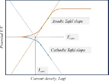
The corrosion current density was determined using the Tafel extrapolation method applied to potentiodynamic curves [12]. By extrapolating the anodic and cathodic slopes from the linear polarization region, the intersection point was identified to determine the corrosion current density, as illustrated in Figure 1. This analysis was facilitated by the EC-Lab® Software integrated into the electrochemical equipment. The corrosion rate, expressed in mils penetration per year (mpy), was then computed using Equation (1) following Faraday's law.
| (1) |
where λ is 1.2688×10⁵, Icorr. is corrosion current density, ρ is the density (7.86g/cm3), and ϵ is the equivalent weight (27.56).
2.5. Data Set
This study utilized potentiodynamic data from polarization curves. Each curve consists of 100 data points representing potential versus current density. A single polarization curve is characterized by four inputs: temperature, pH, salinity concentration, and polarization potential, with the output being the current density. Consequently, the dataset used in this study includes a total of 2700 columns of input and output variables. Each input variable has been normalized to have a value between 0 and 1, as per Equation (2).
| (2) |
where X is the normalized value, x is the unnormalized value, and xmax and xmin denote the maximum and minimum values for each level, respectively.
2.6. Artificial Neural Network, ANN
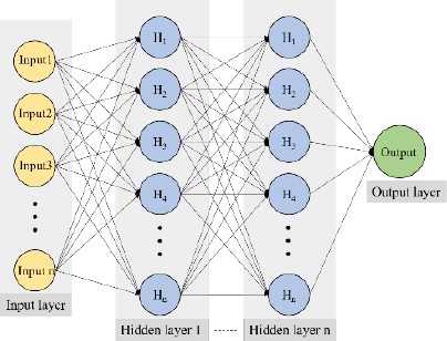
The ANN model employs supervised learning through the back-propagation algorithm. In this study, it is designed to accept four inputs: temperature, pH, salinity concentration, and polarization potential. It then produces an output corresponding to the corrosion current density. As illustrated in Figure 2, the ANN architecture is a multilayer perceptron, consisting of an input layer with four nodes, several hidden layers, and a single-node output layer. The activation function used in each hidden layer is the hyperbolic tangent (tanh) as given by Equation (3).
| (3) |
For the ANN, the data was split into training, validation, and test sets in proportions of 80%, 10%, and 10%, respectively. This division was randomly executed during the training phase. The ANN was implemented in Python 3.7, using the TensorFlow 2.0 library.
3. Results and Discussion
3.1 Potentiodynamic Curves
To generate training data for the ANN model, potentiodynamic tests were performed with factor combinations, as listed in Table 2. The results for the 27 conditions are depicted in Figure 3. All curves illustrate a rapid increase in the current density in the anodic range, which is attributed to the oxidation reaction on the WE. Some curves displayed stagnation in the corrosion current density in the cathodic section owing to oxygen concentration limitations. This phenomenon is known as "oxygen concentration polarization,” indicating that the current density plateaus approximately at 10-1 mA/cm2, which results from oxygen diffusion constraints within the cathodic range [13]. Consequently, the polarization curves revealed complex patterns influenced by factor variables and electrochemical reactions.
Table 3 lists the Icorr., Ecorr., and mpy values obtained using the Tafel extrapolation method. The samples exhibited an mpy range from a minimum of 9.7 to a maximum of 192.8. Factors had varying influences based on the mean and variance of the response. The order is as follows: factor B (pH), factor A (temperature), and factor C (salt conc.).
This suggests that each factor and its level affect both the polarization curve and the corrosion characteristics. Consequently, they can serve as inputs for the ANN to produce significant outputs.
3.2 Optimal Parameters of ANN
Determining the optimal parameters for the ANN model is significant to ensure superior performance during the training, validation, and test phases. These parameters can depend on various factors including the network structure, activation function, learning rate, and data acquisition. Finding the optimal combination typically involves multiple iterations and adjustments. In our study, we employed an ANN with a 4-50-50-1 architecture. The mean squared error (MSE), as presented in Equation (4), was the chosen loss function for training the model.
| (4) |
where, n is the number of outputs for the training set, X(t) is the actual value, and X′(t) is the predicted value. The MSE is used as a loss function for the regression results in the ANN model and represents the difference between the actual and predicted values. Consequently, one of the primary objectives of model training is to minimize MSE through iterative learning.
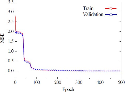
Figure 4 depicts the MSE in relation to the number of epochs for the ANN model. The MSE decreased sharply up to 100 epochs, after which the reduction proceeded more gradually. At a maximum of 500 epochs, the MSE values were found to be 0.0018 and 0.0016, with no further significant decline beyond more epochs. This trend suggests that the ANN model reached an optimal level of training at approximately 100 epochs, where additional training did not markedly enhance the performance.
3.3 Validation for ANN model
Figure 5 illustrates both the actual and predicted curves. For a total of 27 polarization curves, the ANN presented curves that closely resembled the actual shape, as Figure 5(a)-(c).
However, as observed in experiments no. 6 and 19, there were slight deviations at some data points. The ANN showed a very high learning performance on the entire training dataset; however, the cathode region exhibited a slightly lower learning performance than the anode region. Given that ANN models are trained to minimize the loss function, they may emphasize learning in certain regions over others, depending on the range or distribution of the output value [14]. In this study, the output of the ANN model was the current density. The current density in the anodic region in the data was up to two orders of magnitude higher than that in the cathodic region. Therefore, it is possible that the ANN model was trained to preferentially reduce the MSE for the data in the anode region.
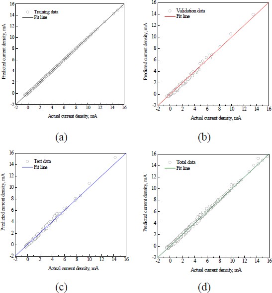
Figure 6 illustrates the correlation between the actual values and ANN’s predictions, providing empirical evidence of the model's performance across the training, validation, and test data. Most data points were concentrated near the best-fit regression line (Y=T), demonstrating a high correlation, with a coefficient of determination close to 1. The correlation coefficients R2 for the training, validation, and test phases were 0.999, 0.9847, and 0.984, respectively, indicating a robust model fitness. Although there are minor deviations between the actual and predicted data at specific points, the overall predictions were consistent and reliable. This indicates the potential of the ANN model to learn the pattern of the polarization curve in complex combinations of factors.
However, a high degree of correlation coefficient might indicate a potential risk of overfitting. Overfitting means that the model might be too closely tailored to the training data, leading to decreased performance with new data. Therefore, external validation using datasets that are not included in the training phase is essential.
3.4 Prediction Performance
Figure 7 shows a comparison of the actual polarization and prediction curves from the ANN model for the new test conditions excluded from the ANN training data. For Test Condition 3 in Figure 7(c), the ANN generated a polarization curve that was very similar to the actual curve. In addition, Ecorr. and Icorr. also showed very similar values, and the actual and predicted mpy values were found to be 42.109 and 35.369, respectively. In contrast, test conditions 1 and 2, illustrated in Figure 7(a, b), exhibited similar Ecorr. values However, a noticeable deviation in the current density between the anode and cathode is evident. This deviation is further emphasized by the significant mpy variation displayed in Figure 7(d). Such outcomes underline the capacity of the ANN model to yield precise predictions for certain Test Conditions, while also revealing its limitations under other conditions, such as Test Conditions 1 and 2.
The observed discrepancies can be attributed to inherent differences or potential noise in the test conditions, suggesting the need for more extensive data collection and model optimization. In summary, the ANN model in its present configuration demonstrates considerable capability in corrosion prediction, particularly in reproducing polarization curves, while emphasizing the need for ongoing optimization to enhance its wider application.
4. Conclusion
In this study, we employed an ANN model to analyze the corrosion patterns of carbon steel based on potentiodynamic tests conducted within a structured experimental matrix defined by a three-level full factorial design. This systematic approach produced 27 distinct polarization curves, each containing 100 data points covering variables such as the temperature, pH, salinity, and polarization potential. Overall, this provided a robust dataset of 2700 data points for training and optimizing our ANN model.
The results demonstrated that the ANN model exhibited robust learning performance in predicting the polarization curve patterns of carbon steel, especially when exposed to environments influenced by a combination of various conditions. In this study, the ANN model displayed notable accuracy, with a correlation coefficient exceeding 0.98 between the training dataset and the predicted outcomes. However, when analyzing data points outside the scope of the training set, the model showed significant discrepancies. It is thus clear that ANNs possess the capability to address the complexities of predicting corrosion behaviors, especially in settings marked by diverse environmental conditions. To further enhance the precision of the ANN model, ongoing efforts focusing on expanding training datasets, improving data preprocessing techniques, and optimizing the model's architecture remain essential.
Acknowledgments
This work was supported by the ‘Autonomous Ship Technology Development Program (20011164, Development of Performance Monitoring and Failure Prediction and Diagnosis Technology for Engine System of Autonomous Ships)’ funded by the Ministry of Trade, Industry & Energy (MOTIE, Korea).
Author Contributions
Conceptualization, K. H. Jung and J. H Lee; Methodology, K. H. Jung; Software, K. H. Jung; Validation, K. H. Jung; Formal Analysis, K. H. Jung; Investigation, K. H. Jung; Resources, J. H Lee; Data Curation, K. H. Jung; Writing—Original Draft Preparation, K. H. Jung; Writing—Review & Editing, J. H Lee; Visualization, K. H. Jung; Supervision, J. H Lee; Project Administration, J. H Lee; Funding Acquisition, J. H Lee.
References
-
X. Hou, L. Gao, Z. Cui, and J. Yin, “Corrosion and protection of metal in the seawater desalination,” IOP Conference Series: Earth and Environmental Science, vol. 108, no. 2, p. 022037, 2018. [Online]. Available: https://iopscience.iop.org/article/10.1088/1755-1315/108/2/022037/meta
[https://doi.org/10.1088/1755-1315/108/2/022037]

-
X. Jiang, Y. Yan, and Y. Su, “Data-driven pitting evolution prediction for corrosion-resistant alloys by time-series analysis,” npj Materials Degradation, vol. 6, no. 1, p. 92, 2022. [Online].
[https://doi.org/10.1038/s41529-022-00307-4]

-
C. Wang, W. Li, Y. Wang, X. Yang, and S. Xu, “Study of electrochemical corrosion on Q235A steel under stray current excitation using combined analysis by electrochemical impedance spectroscopy and artificial neural network,” Construction and Building Materials, vol. 247, p. 118562, 2020. [Online].
[https://doi.org/10.1016/j.conbuildmat.2020.118562]

-
Y. Liu, X. Han, L. Kang, and Q. Li, “Prediction of corrosion rates of Ni-TiN composite coating using a radial basis function neural network,” International Journal of Electrochemical Science, vol. 17, no. 6, p. 220626, 2022. [Online].
[https://doi.org/10.20964/2022.06.15]

-
J. Y, Park and B. S Seo, “A study on resilient back-propagation neural network model for estimation of welding properties of flux cored wire,” Journal of the Korean Society of Marine Engineering, vol. 42, no. 7, pp. 531-538, 2018 (in Korean). [Online]. Available: https://www.e-jamet.org/xml/15811/15811.pdf, .
[https://doi.org/10.5916/jkosme.2018.42.7.531]

-
A. A. Dastgerdi, A. Brenna, M. Ormellese, M. Pedeferri, and F. Bolzoni, “Experimental design to study the influence of temperature, pH, and chloride concentration on the pitting and crevice corrosion of UNS S30403 stainless steel,” Corrosion Science, vol. 159, p. 108160, 2019. [Online].
[https://doi.org/10.1016/j.corsci.2019.108160]

-
A. H. Alamri, “Localized corrosion and mitigation approach of steel materials used in oil and gas pipelines–An overview,” Engineering Failure Analysis, vol. 116, p. 104735, 2020. [Online].
[https://doi.org/10.1016/j.engfailanal.2020.104735]

-
F. Arjmand and A. Adriaens, “Influence of pH and chloride concentration on the corrosion behavior of unalloyed copper in NaCl solution: A comparative study between the micro and macro scales,” Materials, vol. 5, no. 12, pp. 2439-2464, 2012. [Online].
[https://doi.org/10.3390/ma5122439]

-
C. G. Soares, Y. Garbatov, A. Zayed, and G. Wang, “Influence of environmental factors on corrosion of ship structures in marine atmosphere,” Corrosion Science, vol. 51, no. 9, pp. 2014-2026, 2009. [Online].
[https://doi.org/10.1016/j.corsci.2009.05.028]

-
M. T. Gudze and R. E. Melchers, “Operational based corrosion analysis in naval ships,” Corrosion science, vol. 50, no. 12, pp. 3296-3307, 2008. [Online].
[https://doi.org/10.1016/j.corsci.2008.08.048]

-
A. Heyer, F. D'Souza, C. F. Leon Morales, G. Ferrari, J. M. C. Mol, and J. H. W. de Wit, “Ship ballast tanks a review from microbial corrosion and electrochemical point of view,” Ocean Engineering, vol. 70, pp. 188-200, 2013. [Online].
[https://doi.org/10.1016/j.oceaneng.2013.05.005]

- D. A. Jones, Principles and Prevention of Corrosion, 2nd edition: Prentice Hall, 1996.
-
X. L. Zhang, Z. H. Jiang, Z. P. Yao, Y. Song, and Z. D. Wu, “Effects of scan rate on the potentiodynamic polarization curve obtained to determine the Tafel slopes and corrosion current density,” Corrosion Science, vol. 51, no. 3, pp. 581-587, 2009. [Online].
[https://doi.org/10.1016/j.corsci.2008.12.005]

- A. H. Jiang, D. L. K. Wong, G. Zhou, D. G. Andersen, J. Dean, G. R. Ganger, and et al., “Accelerating deep learning by focusing on the biggest losers,” arXiv preprint arXiv:1910.00762, , 2019. [Online].


